Demystifying eta reduction in Excel

If ever there were a term that sounded more confusing that it is, it would be eta reduced lambda. It sounds like something involved in advanced chemistry. But the truth is, it’s simply a technique where Excel automatically fills in the arguments of specific functions.

Eta reduced lambdas are considered an advanced topic, because they require a solid grasp of many other advanced topics.

However, in this article we are cutting out the advanced theory and going straight to the application. Once you see it in action, you will realize it’s not as complex as it sounds.

Starting with the basics

Let’s start really basic. The SUM function.

SUM is one of the first functions we learn, so I’m pretty sure you’ve used it before.

SUM can handle up to 255 different arguments in a single calculation. The example below shows how to use SUM with just 2 arguments. It takes the ranges A1:A4, C1:C4, and sums the result.

=SUM(A1:A4,C1:C4)

As we work through the coming sections, just keep in mind that SUM is a function that accepts multiple arguments.

Introducing BYROW

In the screenshot below there are values in A1:D4. Let’s suggest we want to calculate the total for each row.

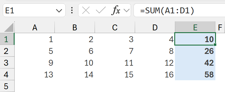
Using traditional Excel methods, we can enter =SUM(A1:D1) into cell E1 and drag the formula down.

This creates 4 separate formulas, one for each row.

Instead, we could use a function like BYROW.

BYROW is a “looping” function; it performs a calculation for each row and returns all the results.

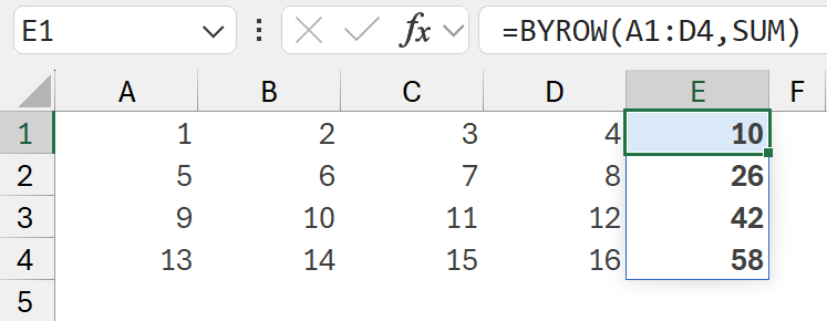
The formula in cell E1 is:

=BYROW(A1:D4,SUM)

This formula applies eta reduction using the SUM function.

In the background, Excel takes the range A1:D4 and performs a calculation on a row-by-row basis.

• The first calculation is: SUM(A1:D1)
• The second calculation is: SUM(A2:D2)
• The third calculation is: SUM(A3:D3)
• The third calculation is: SUM(A4:D4)

BYROW takes the whole array, slices it into rows, then passes each row into the SUM function.

The results are returned in a single cell that spills into the other cells below. We don’t need to copy or drag any formulas.

In this scenario, SUM doesn’t need any brackets or arguments. Excel assumes the values used in SUM are the values passed across by the BYROW function.

This is eta reduction in action.

BYCOL works in the same way but passes across the values in each column.

You can learn more about BYROW and BYCOL in Tip #497.

Introducing MAP

In the screenshot below we have 2 ranges, A1:D4 and A7:D10. Let’s suggest we want to SUM the individual cells in each range based on the relative cell positions.

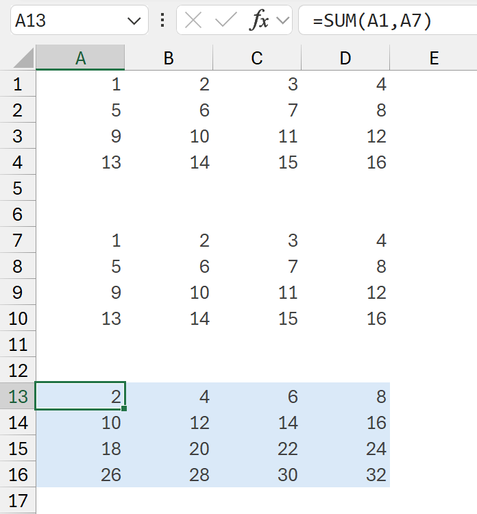
The formula in cell A13 is:

=SUM(A1,A7)

Using traditional Excel methods, we can enter a single formula, then drag that formula into the other cells as required.

In this scenario, we could also use MAP, it is another looping function.

Where BYROW calculated row by row, MAP handles multiple arrays and calculates cell by cell.

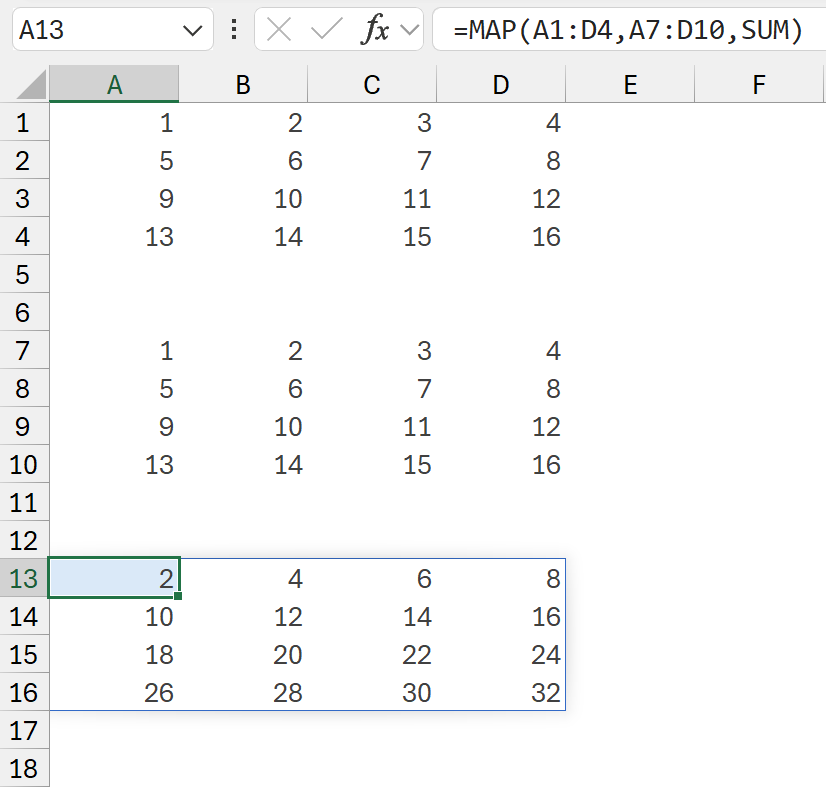
The formula in cell A13 is:

=MAP(A1:D4,A7:D10,SUM)

This formula also applies eta reduction using the SUM function.

In the background, Excel takes the ranges A1:D4 and A7:D10 and performs a calculation based on the relative position of each value in the arrays.

• The first calculation is: SUM(A1,A7)
• The second calculation is: SUM(B1,B7)
• The third calculation is: SUM(C1,C7)
• And so on.

The MAP function takes both arrays, and slices them into cells, it then passes the cells from each array into the SUM function.

Each cell calculates and returns in a single result, which spills into the other cells; no formula dragging required.

Once again, SUM doesn’t need any brackets or values, because using eta reduction, Excel assumes the values from the first array are used in the first argument of SUM, and the values passed from the second array are used in the second argument.

Other functions

We have seen that eta reduction works well with SUM. But it can work with other functions that returns a single value.

Let’s take TEXTJOIN for example.

TEXTJOIN combines text from multiple ranges with a delimiter between each value.

TEXTJOIN has the following arguments

• Delimiter: The character(s) to place between each value.
• Ignore_empty: Determines if empty cells are treated as values, or ignored
• Text1: The text to join
• [Text2, ...]: Any additional text to join.

In the SUM section above, we noted that MAP:

• Passes the values from the first array into the first argument
• Passes the values from the second array into the second argument

This isn’t limited to two arrays. MAP can handle up to 254 arrays.

Therefore, we can use MAP with the TEXTJOIN function.

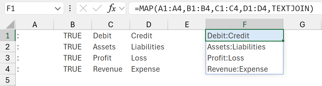
The formula in cell F1 is:

=MAP(A1:A4,B1:B4,C1:C4,D1:D4,TEXTJOIN)

This formula applies eta reduction using the TEXTJOIN function.

It takes the ranges A1:A4, B1:B4, C1:C4, D1:D4 and performs a calculation on a cell-by-cell basis.

• The first calculation is: TEXTJOIN(A1,B1,C1,D1)
• The second calculation is: TEXTJOIN(A2,B2,C2,D2)
• The third calculation is: TEXTJOIN(A3,B3,C3,D3)
• The fourth calculation is: TEXTJOIN(A4,B4,C4,D4)

Once again, this is eta reduction in action. From a single formula in F1, it spills the results into the other cells.

The TEXTJOIN example works with eta reduction because there are 4 arrays in the MAP function, and TEXTJOIN can work with 3 or more arguments.

But we can’t use eta reduction where there is a mismatch.

• BYROW(A1:A4,LEFT) will not work because BYROW passes 1 argument, but LEFT requires 2.
• MAP(A1:A4,B1:B4,LEFT) will work because MAP will pass 2 arguments and LEFT also requires 2 arguments.

Looping functions

Eta reduction works with all looping functions (also known as LAMBDA helper functions).

We have already seen:

• BYROW passes across 1 argument.
• MAP passes across arguments based on the number of arrays selected.

But there are other looping functions, and they each pass across values in different ways. The following table shows the different kinds of values passed into the function we provide.

* For GROUPBY and PIVOTBY, if using eta reduction, only the subset argument is passed across. The totalset is used for more advanced functions.

Each eta reduced function only returns a single result, it is the looping function that determines the values passed across and the shape of the result.

Passing eta reduced lambdas as arguments

What makes eta reduced lambdas even more interesting is that we can dynamically switch out different functions.

We can’t enter a function into a cell, but we can include it within a formula.

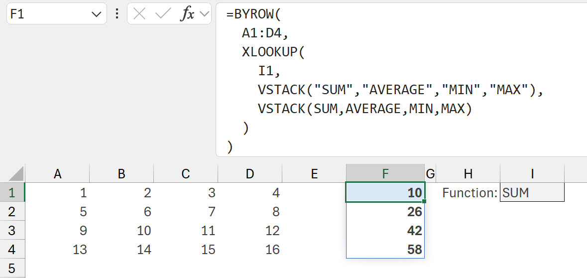
The formula in cell F1 is:

=BYROW(
  A1:D4,
  XLOOKUP(
    I1,
    VSTACK("SUM","AVERAGE","MIN","MAX"),
    VSTACK(SUM,AVERAGE,MIN,MAX)
  )
)

The XLOOKUP looks in cell I1, and checks if it equals the text of "SUM", "AVERAGE", "MIN" or "MAX". If it does, it returns the SUM, AVERAGE, MIN, or MAX as a function.

Then, this function is used inside BYROW. So, if a user changes the value in I1 from "SUM" to "AVERAGE", the row-by-row calculation will change to an AVERAGE. Therefore, users can decide which aggregation they wish to see.

Conclusion

Eta reduction is a powerful technique to avoid complex LAMBDA functions. They provide the ability to use standard Excel functions directly inside looping functions like BYROW, MAP, etc. Once we understand what each looping function passes in, we can simplify even advanced array calculations. It’s a subtle technique, but one that opens up new ways to work with Excel.