Reduce spreadsheet maintenance with a dynamic total row

Ever since the introduction of dynamic array calculations in Excel, one of the most common questions from finance users is: “How can I add a total at the bottom?”

It’s a good question because nobody wants to keep updating their formulas. Let’s answer this question in this article.

GROUPBY & PIVOTBY

Before we start looking at anything with multiple functions, there is good chance you can get everything you need from the GROUPBY and PIVOTBY functions.

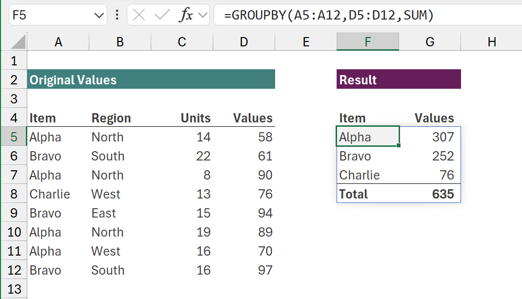
The formula in cell F5 is:

=GROUPBY(A5:A12,D5:D12,SUM)

• Row_fields (A5:A12) - The values to group the rows by.
• Values (D5:D12) - The values to aggregate.
• Function (SUM) - The calculation to perform on the values.

As you can see from the screenshot above, this is a single function which has successfully grouped the data and included a total row at the bottom.

If we want to aggregate vertically and horizontally, we can use the PIVOTBY function.

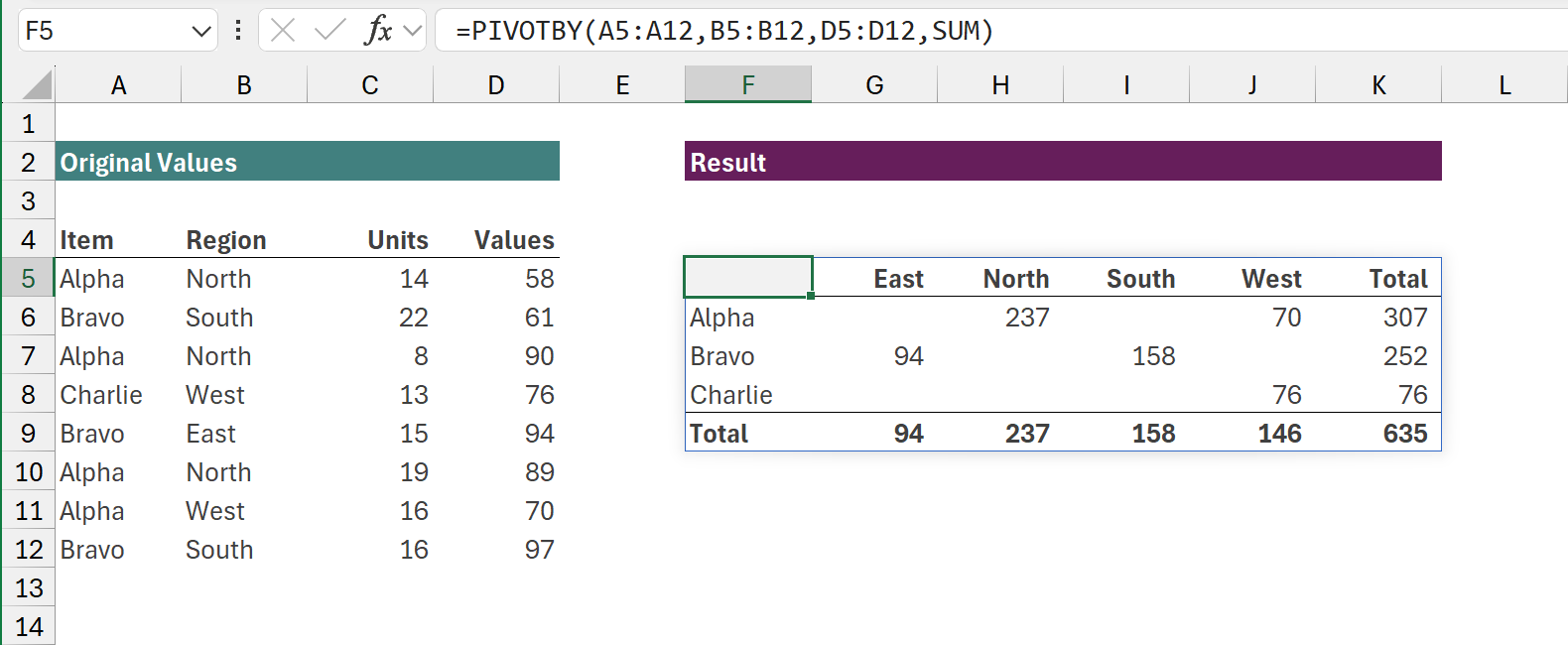
=PIVOTBY(A5:A12,B5:B12,D5:D12,SUM)

The arguments used in the PIVOTBY are:

• Row_fields (A5:A12) - The values to group the rows by.
• Col_fields (B5:B12) - The values to group the columns by.
• Values (D5:D12) - The values to aggregate.
• Function (SUM) - The calculation to perform on the values.

By default, there will be a total row at the bottom.

GROUPBY and PIVOTBY are great solutions if we want to group and aggregate the data. But if that isn’t our use case, we need a different approach. That’s what we will look at in the next section.

Add a total row to any array calculation

By using the right techniques, we can add a total row to any array result. For our example we will use the FILTER function to illustrate this.

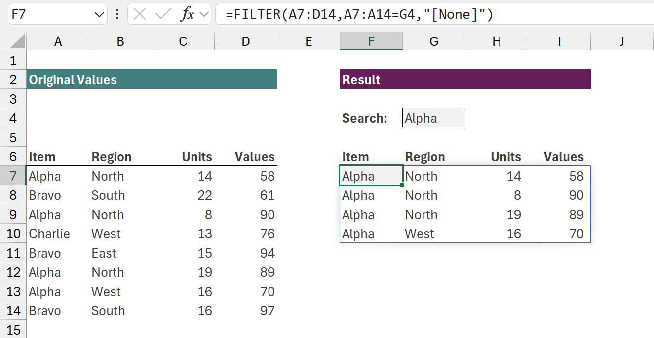
The formula in cell F7 is:

=FILTER(A7:D14,A7:A14=G4,"[None]")

This uses the FILTER function to return only the rows where A7:A14 are equal to Alpha.

Alpha has 4 records; Bravo has 3 and Charlie has 1. Therefore, the number of results will change depending on the item selected in G4.

Practical approach - totals at the top

There is a simple way to avoid all the complexity... place the totals at the top.

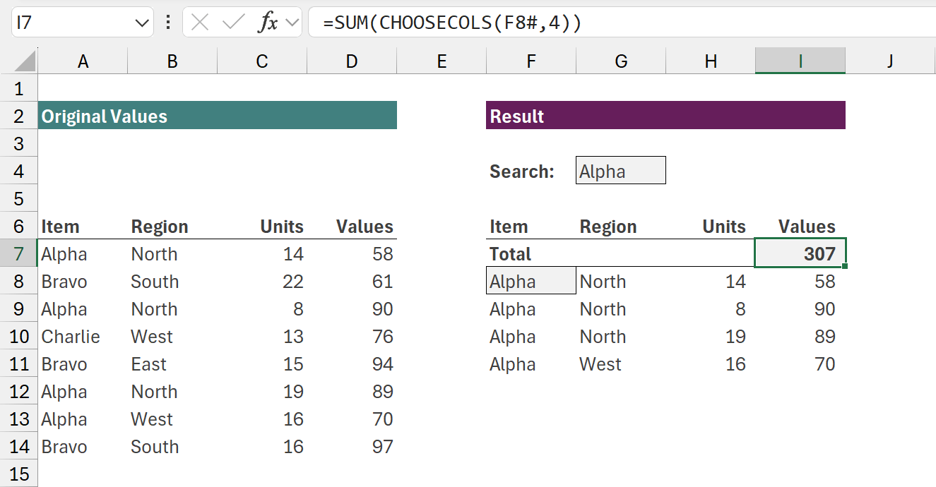
The formula in cell I7 is:

=SUM(CHOOSECOLS(F8#,4))

Since the total row is always at the top, we don’t need to worry about it moving.

The result of the FILTER function is in cell F8. Therefore, using CHOOSECOLS(F8#,4), takes all the values from the FILTER and selects only the 4th column. These values are then passed into to SUM function to calculate the total.

While this approach is easy, it’s not what most of us are familiar with. Just based on our school days, we were taught that totals go at the bottom. So, let’s look at that next.

The common approach - totals at the bottom

To create a total row at the bottom which moves automatically, we can’t insert the total row into a specific cell. Instead, we incorporate it into the formula itself.

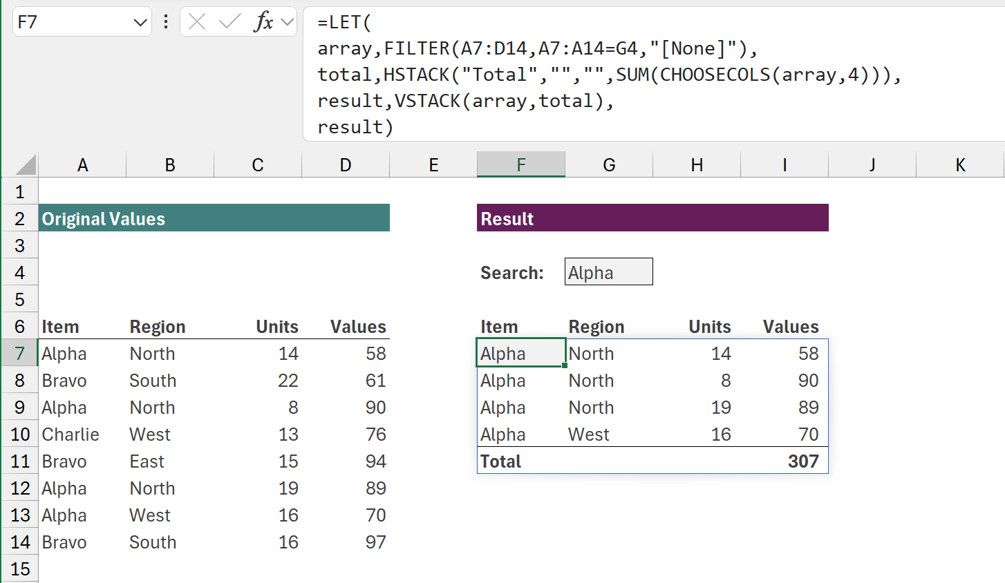
The formula in cell F7 is:

=LET(
array,FILTER(A7:D14,A7:A14=G4,"[None]"),
total,HSTACK("Total","","",SUM(CHOOSECOLS(array,4))),
result,VSTACK(array,total),
result)

In this example, we use the LET function to give names to each calculation. Then we re-use the names later in the calculation.

• Array: The result of the FILTER function we saw at the start of this section.
• Total: Uses HSTACK to create an array which has the same number of columns as the FILTER calculation. Column 1 contains the word “Total”, Columns 2 and 3 are empty text strings, Column 4 uses the SUM / CHOOSECOLS combination to aggregate only the 4th column.
• Result: Uses VSTACK to combine the array and total calculations into a single result.
• The last argument of LET states which values to return. We are returning the result value.

We now have a total row at the bottom. It doesn’t matter how many rows there are, the total will always be at the bottom.

How to format a total row?

If you try this in your workbook, you will soon discover the total doesn’t look like a total. It’s not bold and there is no border. Unfortunately, formatting is associated with the cell, and not the value in the cell. Therefore, to format the total we must apply conditional formatting.

1. Select the maximum range of cells the formula result could occupy. This will start at F7 which is the first cell.
2. From the ribbon, click Home > Conditional Formatting > New Rule...

3. In the New Formatting Rule window select Use a formula to determine which cells to format
   In the formula box enter the following:

   =$F7="Total"

   The selected cells start at F7; therefore, this will format the row where the text in column F is equal to “Total”.

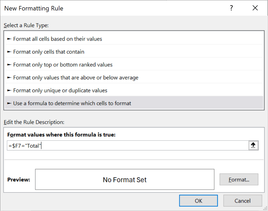
4. Click the Format button and apply the relevant formatting. For my screenshots, I’ve chosen bold text and top border. Then click OK.
5. Click OK.

You now have formatting applied to the cells.

If we change the Search from Alpha to Bravo the total appear to move. Alpha had 4 items, with the total in row 11. Bravo has 3 items; therefore, the total is now in row 10.

Once the formula is set up, the total row moves automatically.

Conclusion

In this article, we saw how we can remove the need to update a total row. Using dynamic array calculations, the total row now moves automatically depending on how many values returned in the calculation. Now we can be more efficient, as we don’t need to update our workbooks as often.