Running totals in filtered tables

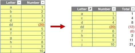
Here is a common problem for anyone that uses cumulative / running total reports frequently. We often want to write a formula in a new column of a created (CTRL + T) Table to calculate the running total of a column (let’s call the field Number) regardless of whether the Excel Table is filtered or not.  The result should look like the column Total generated on the right (below):

Normally, we would think of using SUM to sum up a range in Excel from the top row to the current row to calculate the running total.  However, the result will not be adjusted if the table is filtered or it will be adjusted incorrectly if rows are added in the middle of the Table.

Hence, we think of using an Excel function that ignores any rows that are not included in the result of a filter.  That function is SUBTOTAL.  But I’m getting ahead of myself!

Firstly, the current row of column Number can be easily identified using the Table reference as below.

=[@Number]

This form of syntax is known as “structured referencing”.  You may also recall the @ symbol denotes the implicit intersection (i.e. an item either on the same row or the same column) and literally means the value of the Number field for the row you are on.

Secondly, we can easily select a range from the top row to current row and anchor the top row reference.  However, that will be insufficiently flexible if the top row is deleted or a new row is added at the start.  Therefore, we use INDEX to find the top cell of the ‘Number’ field as follows.

=INDEX([Number],1)

You may recall INDEX(array, row_number, [column_number]) returns a value or the reference to a value from within a table (array) or range (list).  For example, INDEX({7,8,9,10,11,12},3) returns the third item in the list {7,8,9,10,11,12}, i.e. 9.  This could have been a range: INDEX(A1:A10,5) gives the value in cell A5, etc.

Using it in reference form, this means you can use it along with a colon, “:”, to refer to a range of cells.  This is precisely what we require.  The range that we need for the running total is as follows:

=INDEX([Number],1):[@Number]

This defines the range from the first entry in the field Number to the current entry in that same field.

Finally, we then use SUBTOTAL to generate the running total.  At first glance, SUBTOTAL seems like many other Excel functions:

=SUBTOTAL(function_number, ref1, ref2, …)

Here, the function_number is an integer between one [1] and 11 inclusive, or 101 and 111 inclusive, as follows:

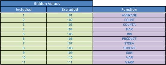
For the function_number constants from one [1] to 11, the SUBTOTAL function includes the values of rows hidden by the ‘Hide Rows’ command.  These constants should be used when you want to subtotal hidden and unhidden (visible) numbers in a list.  For the function_number constants from 101 to 111, the SUBTOTAL function ignores values of rows hidden by the ‘Hide Rows’ command.  These constants should be used when you want to subtotal the visible numbers in a list only.

SUBTOTAL ignores all filtered rows regardless of which function number in the first argument is used.  Filtering should not be confused with hiding!

=SUBTOTAL(9,INDEX([Number],1):[@Number])

The number nine [9] represents the SUM function including hidden rows whilst number 109 works similarly but ignores hidden rows.  These hidden rows need to be caused by either hiding or grouping (not filtering).  Depending upon your purpose for the running total, you can choose which number to use.