
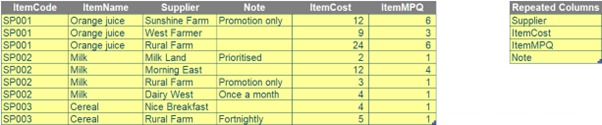
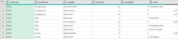
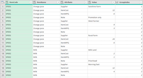
For the second month running, I have an article inspired by recent consulting problems. Obviously, I will change the data! Imagine we have a table called Data (sorry, that’s as far as my imagination goes!) that contains details of some new items and their suppliers in a standard tabular format (i.e. a vertical list), as below. Let’s suppose we need to import this data into an inventory management system.

We need to convert this automatically such that when the data updates, it will be trivia to refresh. Therefore, this month I shall branch out in the wonderful world of Get & Transform (i.e. The Artist Formerly Known As Power Query) in order to transform the structure of the data from the original vertical format to the required horizontal one.
You can download the example file here.
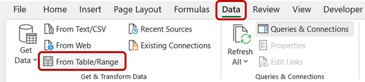
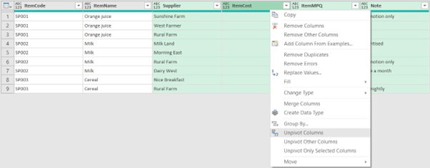
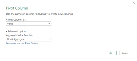
Firstly, we will import the two Tables into Power Query, one by one, by selecting each Table and then navigating to the Data tab, and click ‘From Table/Range’ under the ‘Get & Transform Data’ grouping, viz.

We need Power Query to identify a list of grouped columns (i.e. ItemCode and ItemName). To do this, we add a new step by clicking ‘fx’ next to the Formula bar. Then, we will use Power Query’s List.RemoveItems and Table.ColumnNames functions to remove all repeated columns listed in the Column list (which we created earlier) from the Source step. We add the formula below to the Formula bar and name this step as GroupCols.
=List.RemoveItems(Table.ColumnNames(Source),Column)

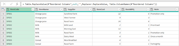
Then, we re-order the columns with the following formula. List.Combine helps combine grouped columns above with the Column list, which has a correct column order for repeated columns.
=Table.ReorderColumns(#“Replaced Value”,List.Combine({GroupCols, Column})
As you can see from the picture below, Note is now the last column:
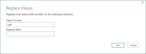
To keep the query dynamic, we need to replace the grouped columns with our variable ‘GroupCols’ from:
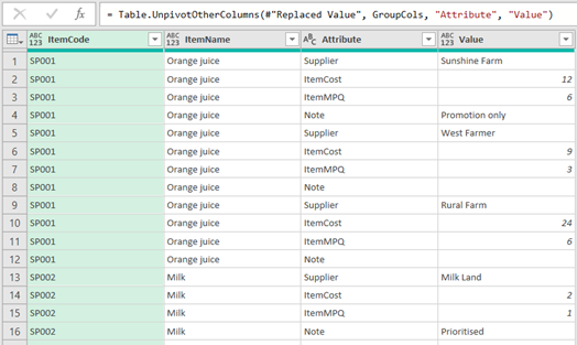
= Table.UnpivotOtherColumns(#"Replaced Value", {"ItemCode", "ItemName"}, "Attribute", "Value")
into:
= Table.UnpivotOtherColumns(#"Replaced Value", GroupCols, "Attribute", "Value")
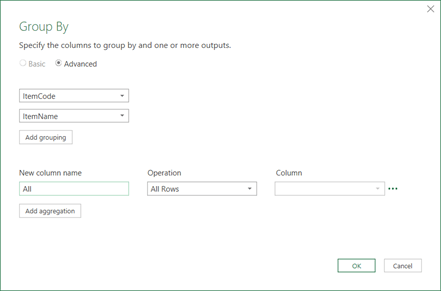
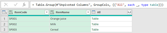
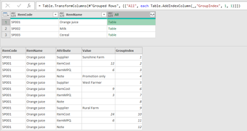
We are then going to add an index column in each table within the All column, such that when it reaches a row with new ItemCode and ItemName values, the index resets to one [1]. We then create a new blank step called Indexed and apply the following formula:
= Table.TransformColumns(#"Grouped Rows", {{"All",
each Table.AddIndexColumn(_,"GroupIndex", 1, 1)}})

While the above indexing would allow us to separate the data based on each item code and name, we would like to further index and separate the data by suppliers as well. First, we need to establish the number of repeated columns or the number of rows per unique supplier, which is four [4]. To do this, we use List.Count function as below:
=List.Count(Column)
We will rename this step as RepeatedCols, and next we use the following formula for a new blank step:
= Table.TransformColumns(#"Expanded All", {{"GroupIndex", each Number.RoundUp(_ / RepeatedCols), type number}})
The above formula rounds up the index column to the closest division of four, e.g. 1/4 = 0.25 rounded up is one [1], 2/4 = 0.5 rounded up is still one [1] etc. Thus, the query will now look like this:


It may seem like a lot of work, but now, when the data updates, all you have to do is ‘Refresh’.
The Final Friday Fix will return on Friday 27 May 2022 with a new Excel Challenge. In the meantime, please look out for the Daily Excel Tip on our home page and watch out for a new blog every business working day.
Archive and Knowledge Base
This archive of Excel Community content from the ION platform will allow you to read the content of the articles but the functionality on the pages is limited. The ION search box, tags and navigation buttons on the archived pages will not work. Pages will load more slowly than a live website. You may be able to follow links to other articles but if this does not work, please return to the archive search. You can also search our Knowledge Base for access to all articles, new and archived, organised by topic.
