What is scalar lifting, and why should you care?

When Microsoft introduced the dynamic array calculation engine for Excel in 2018, it completely changed how Excel calculates values. One of the key elements was Excel’s handling of scalar lifting!

I know what you’re thinking... “What on earth is scalar lifting?”

Scalar lifting impacts almost every function. It is a key concept of how Excel works. Yet, most users have never heard of it and have no idea how important it is.

So, in this article we explore what it is and why it matters. This article explores more complex concepts in Excel and so may be geared towards those with Creator and Developer level competencies. You can read more about our spreadsheet competency framework here.

What is a scalar?

Scalar lifting is two technical terms brought together in a single name. Let’s start by understanding the first: Scalar.

In computing, a scalar is simply a single value, such as a number or a text value. For example, 100 is a scalar, “ICAEW” is a scalar.

That’s it! It’s that simple.

Scalars are important to Excel because of how functions use them.

Let’s look at an example with a function that most have used at some point: VLOOKUP.

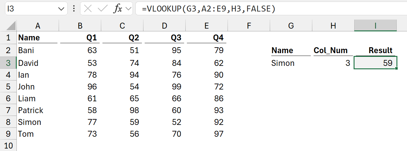
The formula in cell I3 is:

=VLOOKUP(G3,A2:E9,H3,FALSE)

In the range A2:E9, we are looking up the value of Simon in the first column and returning the value from the 3rd column. The last value is FALSE because we want an exact match.

The function definition for VLOOKUP is:

VLOOKUP (lookup_value, table_array, col_index_num, [range_lookup])

• lookup_value is the value to look up from the first column of the table_array.
• table_array is the range of cells to search for the lookup_value and provide the return value.
• col_index_num is the column number to return the value from.
• range_lookup is a logical value to specify if the function performs an approximate match (TRUE) or an exact match (FALSE).

Of these function arguments, some expect single values (ie, scalar values), and some expect multiple values (non-scalar values).

The function arguments which are scalar or non-scalar are not documented anywhere. But, when we know a little bit about a function, it’s pretty easy to work out which is which. In the case of VLOOKUP:

Scalar

• lookup_value is scalar because we look up a single value.
• col_index_num is scalar because we return the value from a single column.
• range_lookup is scalar because we provide a single TRUE/FALSE value.

Non-scalar

• table_array is not scalar, it will always have multiple values.

We can apply this concept of scalar and non-scalar arguments to nearly all functions in Excel. The exceptions are those with zero arguments such as TODAY, RAND, etc.

What is lifting?

Having looked at the meaning of Scalar, let’s now turn our attention to the second term: Lifting.

Lifting occurs when a function argument which expects a single value is provided with multiple values. When this occurs, the function performs a calculation for each value and returns multiple results.

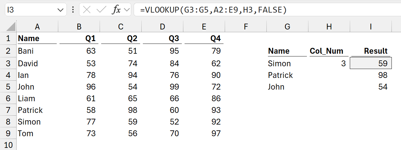
The formula in cell I3 is:

=VLOOKUP(G3:G5,A2:E9,H3,FALSE)

As noted above, lookup_value is a scalar argument, it expects a single value. Yet, in this example we provide multiple values.

We might expect Excel to return an error, but it doesn’t. Instead, it performs the calculation for all the values.

We are telling Excel to:

• Use the range A2:E9, look up the value of Simon in the first column, and return the value from the 3rd
• Use the range A2:E9, look up the value of Patrick in the first column, and return the value from the 3rd
• Use the range A2:E9, look up the value of John in the first column, and return the value from the 3rd

Excel returns all three values.

This isn’t us creating a formula and dragging down. Excel calculates all three results from a single formula. Only cell I3 has a formula. I4 and I5 display the results calculated in I3.

This is lifting in action.

With it, we can replace hundreds, thousands or even millions of formulas with a single formula.

Where else can we apply scalar lifting?

As noted earlier, this concept of scalar lifting applies to almost all Excel functions. Let’s look at another example: SUMIFS.

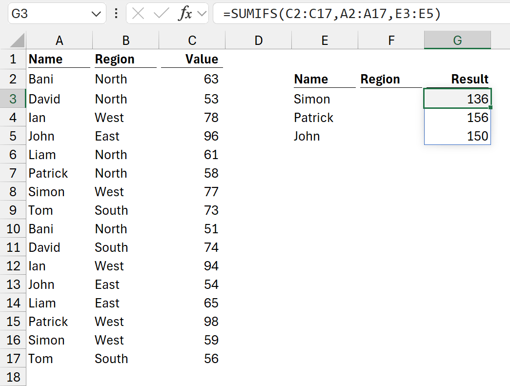
The formula in cell G3 is:

=SUMIFS(C2:C17,A2:A17,E3:E5)

The function definition for SUMIFS is:

SUMIFS(sum_range, criteria_range1, criteria1, [criteria_range2, criteria2], ...)

• sum_range is the range of cells to sum.
• criteria_range1 is the range to test using Criteria1.
• criteria1 is the criteria that defines which rows from criteria_range1 to include in the sum.
• [criteria_range2, criteria2], … are additional optional ranges and their associated criteria.

The scalar and non-scalar arguments are pretty easy to spot:

Scalar

• criteria1 is a scalar because it is the single value we want to check for.

Non-scalar

• sum_range is non-scalar because we provide a range of cells to sum from.
• criteria_range1 is non-scalar because we provide a range of cells to check criteria1 against.

SUMIFS can have optional arguments for criteria_range and criteria, which follow the same pattern:

• The criteria are always scalar
• The criteria_range are always non-scalar.

Using the SUMIFS formula above, we are telling Excel:

• If Simon exists in A2:A17, include the corresponding value from C2:C17 in a sum.
• If Patrick exists in A2:A17, include the corresponding value from C2:C17 in a sum.
• If John exists in A2:A17, include the corresponding value from C2:C17 in a sum.

Excel returns all the values.

Again, this is based on a single formula. Only cell G3 has a formula. G4 and G5 display the results calculated in G3.

Pairwise lifting vs. array of arrays

Both VLOOKUP and SUMIFS can have multiple scalar arguments. So, what happens if we provide multiple values into multiple scalar arguments?

Unfortunately, that’s not as straight forward.

Let’s look back at SUMIFS.

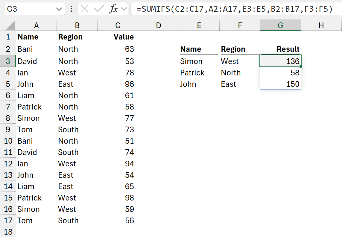
The formula in cell G3 is:

=SUMIFS(C2:C17,A2:A17,E3:E5,B2:B17,F3:F5)

In this example, we have multiple criteria and have provided each with multiple scalar arguments (Simon, Patrick, John for A2:A17, and West, North, East for B2:B17).

In this scenario, the criteria are paired based on their relative position. Excel has paired Simon with West, Patrick with North and John with East.

We are telling Excel:

• If Simon exists in A2:A17 and West exists in B2:B17, include the corresponding value from C2:C17 in a sum.
• If Patrick exists in A2:A17 and North exists in B2:B17,include the corresponding value from C2:C17 in a sum.
• If John exists in A2:A17 and East exists in B2:B17,include the corresponding value from C2:C17 in a sum.

The values in criteria1 and criteria2 are matched based on their relative position. The lifting occurs on both values, so we call this pairwise lifting. We are not restricted to 2 items, we can have any number of criteria, and it would still be called pairwise lifting.

But what if we do something similar with VLOOKUP?

The formula in cell I3 is:

=VLOOKUP(G3:G5,A2:E9,H3:H5,FALSE)

This looks like it performs pairwise lifting, but it’s not.

The values should be:

• Simon from column 3 = 59 – Correct.
• Patrick from column 2 = 58 – But the formula shows 98.
• John from column 4 = 99 – But the formula shows 54.

This doesn’t calculate the value we expect because this is not pairwise lifting. Instead, each argument is lifting separately. As a result, it creates an array of arrays scenario, which only returns the first value from each array.

We have covered the array of arrays problem in a previous article: Solving the array of arrays issue

The values returned by the Excel formula above are:

• Simon column 3 = 59
• Patrick column 3 = 98
• John column 3 = 54

The formula finds the all the values from column 3, column 2 and column 4 but only returns the lookup for Simon, Patrick and John from the first array (column 3).

This is the Array or arrays issue. The results are consistent and predictable, but it is unlikely to provide the value we expect.

For any function, how do we know which treatment we will get? It depends on how the function has been designed.

SUMIFS is specifically designed to work with multiple criteria and therefore performs pairwise lifting. VLOOKUP is designed to work with a single criteria and therefore is not built to work with pairwise lifting.

Just as scalar arguments are not documented; which functions handle pairwise lifting are also not documented. So, if you are unsure, test.

Conclusion

In this article, we’ve seen that functions calculate multiple times if provided with multiple values into arguments which expect a single value.

This underpins how nearly all functions in Excel operate.

Using this approach, we can replace hundreds, thousands or millions of formulas with a single formula.

When there is a single scalar argument the results are reasonably consistent.

However, if there are multiple scalar arguments provided with multiple values, we need to understand how the function has been designed to know whether it performs pairwise lifting or generates an array of arrays.