Automated Grouping

Many of us that prepare spreadsheet reports realise that we have to produce summaries at various levels of granularity.  Some make the mistake of using different worksheets for these reports, but this can cause unnecessary reconciliation issues if things change. Grouping may be a preferred option – which we will come to shortly.

Sometimes when constructing spreadsheets, modellers may want to hide certain data / calculations.  This can be undertaken by formatting the cells or if the rows or columns should be hidden by hiding the necessary rows / columns (CTRL + 9 and CTRL + 0 respectively).

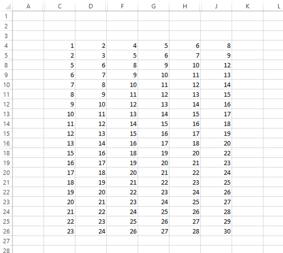
This illustration (above) shows that it can be difficult to spot hidden rows and columns; you have to look at the row and column headers and this presupposes that these are visible.

An alternative to hiding is grouping:

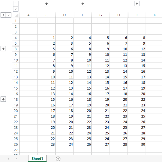
Grouping is undertaken by selecting the row or column (similar to hiding) but then go to the Data tab on the Ribbon and in the Outline section, select the ‘Group’ button and press Group.  The keyboard shortcut is faster and more intuitive: ALT + SHIFT + Right Arrow (whereas ALT + SHIFT + Left Arrow removes the grouping).

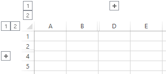
Grouping introduces ‘levels’ to a spreadsheet: in the graphic above, notice how the plus buttons are aligned with the buttons marked ‘Number 1’.  Level 1 is always all grouped sections collapsed.  If all of the plus buttons are pressed, our example would be displayed as follows:

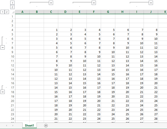
The plus (+) buttons have become minus (-) buttons, still aligned with the ‘Number 1’ buttons.  This is because if you pressed the numbered buttons all of the rows / columns grouped to the same level would be displayed consistently, rather than pressing a multitude of plus and minus buttons.  The hidden rows and columns are easier to identify, and simpler to collapse / expand as required.

Grouping can be taken to eight [8] levels, viz.

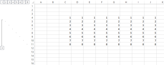
Rows 5 to 11 in this illustration have been grouped at differing levels by holding ALT + SHIFT depressed whilst pressing the Right Arrow key (you can see the dots on the left-hand side of the image before the row headers).  Here, because the rows are next to each other, Excel cannot display separate plus buttons so users would have to use the numbered buttons instead.

The positioning of the plus buttons can be confusing as they actually align with the row / column after the grouping in the default setting:

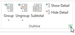
The settings are changed by returning to the Outline section of the Data tab and clicking on the small icon in the bottom right-hand corner (keyboard shortcut, ALT + A + L):

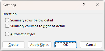
Then, clear both check boxes in the dialog box that appears and then press OK:

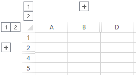
This moves the buttons to the row / column prior to the grouping which, personally, makes more sense to me.

Grouping is very useful in practice. For example, imagine you are a management accountant that has to provide a Gross Profit analysis for your line manager, the Chief Financial Officer and the Board.  It is likely that all three stakeholders will require different levels of detail.  In the past, I have seen many clients prepare three [3] different spreadsheets for these customers, which causes unnecessary re-work and potential reconciliation issues.

This might be a solution which can summarise at those three levels easily:

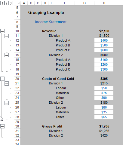
Pressing the numbered buttons will produce all reports required – simple!

With all this borne in mind, it is useful to be able to automate such grouping, as it is a laborious manual task otherwise.  It requires some VBA code, but it is fairly straightforward (i.e. you can copy it).  Consider this screenshot from the attached Excel file:

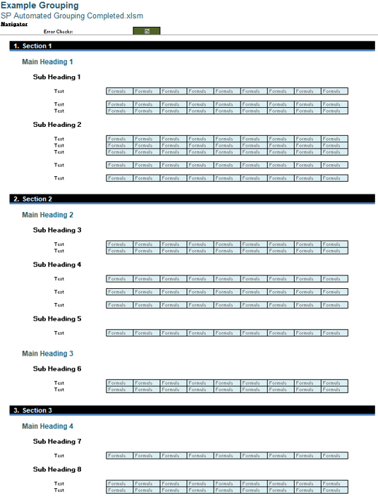
I appreciate it is difficult to read, but the structure is the key concept to get from this image.  We want to group the worksheet as follows, using the structure presented above.

First level:

Second level:

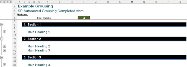
Third level:

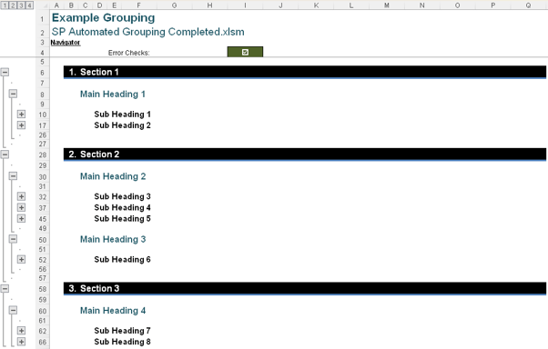
One simple way here is to group all the rows with used range to the highest level and then ungroup each heading at different levels.  I appreciate the remainder of this article may be overkill for some – so feel free to skip and copy the code or else refer to the attached Excel workbook.

The first step is to define the variables for integers and ranges.

Dim rng As Range
Dim firstRow, lastRow as Integer

If there are existing groupings, we need to expand all rows to avoid potential errors in the following sections of code.

ActiveSheet.Outline.ShowLevels RowLevels:=8, ColumnLevels:=8

Next, we define the starting row and the last row of formula by using the UsedRange method to find the first row and use the total count method to find the last row.  The values of rows are assigned to the variables we defined above.

firstRow = ActiveSheet.UsedRange.Row +5
lastRow = ActiveSheet.UsedRange.Rows(ActiveSheet.UsedRange.Rows.Count).Row

Then, we need to unhide all rows (if any) and clear the existing outline for all rows between the starting row and the last row.  Thus, we can remove all existing groupings and get the used range ready for the grouping pattern, as required.

Rows(firstRow & ":" & lastRow).EntireRow.Hidden = False
Rows(firstRow & ":" & lastRow).ClearOutline
On Error Resume Next

Next, we group the rows between first row and last row three [3] times to the fourth [4th] level of grouping.  We group all the rows at highest level of grouping and then we can start to ungroup each heading.  This is more efficient than selectively grouping.

Rows(firstRow & ":" & lastRow).Rows.Group
Rows(firstRow & ":" & lastRow).Rows.Group
Rows(firstRow & ":" & lastRow).Rows.Group

For the third level of headings, we loop through column D.  If the cell’s value in column D is not blank, then we ungroup the row.  Thus, the headings in column D will be grouped at third level.

For Each rng In Range("D" & firstRow & ":D" & lastRow)
    If Not IsEmpty(rng.Value) Then
        rng.Rows.Ungroup
    End If
Next

For the second level of headings, we loop through each range in column C.  If the cell’s value in column C is not blank, then we ungroup the current row twice and use the VBA Offset function to locate the row above and below the current row and ungroup both rows.  Specifically, if there is a heading in column C, we ungroup the row twice to make the headings grouped at second level.

The reason why the rows above the current row need to be grouped is because we need to keep a gap between the first heading and the second heading.  Therefore, the grouping level at this row should be the same as the second level of headings.  As for the rows beneath the current row, we need to ungroup them in order to create the gap between the second level of headings and the third level of headings.

There is also a complication with column C here.  You will notice that it contains 'Heading level 2 Text' style and also 'Heading level 1 Text' style, whereas on column B it only contains 'Heading level 1 Number' style.  Hence we need a simple VBA If here to check if our headings is actually 'Heading level 2':

If IsEmpty(rng.Offset(-2, -1)) Then rng.Offset(-1, 0).Rows.Ungroup

This needs to be inserted at the end of the following code for the heading in column C:

For Each rng In Range("C" & firstRow & ":C" & lastRow)
    If Not IsEmpty(rng.Value) Then
        rng.Rows.Ungroup
        rng.Rows.Ungroup
        rng.Offset(1, 0).Rows.Ungroup
        If IsEmpty(rng.Offset(-2, -1)) Then rng.Offset(-1, 0).Rows.Ungroup
    End If
Next

For the first level of headings, we loop through the column B.  If the cell’s value in column B is not blank, then we ungroup the current row three [3] times to make the headings at first level of grouping.  Again, we use the Offset function to locate the row above and below the current row and ungroup them twice and once respectively.

For the rows above the current row, we need to ungroup twice to make sure that the first levels of headings are adjacent to each other.  For the rows beneath the current row, we ungroup them to keep a gap between the first heading and the second heading.  Also, we use error handling in the loop.

This is because we need to use error handling in this loop so that if there is no outline in the rows defined above, the macro will not return an error and stop at a specific step in the loop.  However, the error handling ensures the macro will ignore the rows without outline and continue grouping until the end of loop.  Finally, the error handling is closed off with ‘GoTo 0’ syntax.

For Each rng In Range("B" & firstRow & ":B" & lastRow)
    If Not IsEmpty(rng.Value) Then
        On Error Resume Next
        rng.Offset(-1, 0).Rows.Ungroup
        rng.Offset(-2, 0).Rows.Ungroup
        rng.Offset(1, 0).Rows.Ungroup
        rng.Rows.Ungroup
        rng.Rows.Ungroup
        rng.Rows.Ungroup
        On Error GoTo 0
    End If
Next

Finally, we point back to the range A1, it helps to reset the worksheet to the top left-hand side.

Range("A1").Select
Putting it all together, we get the following:
Sub rowGrouping()

Dim rng As Range
Dim firstRow, lastRow As Integer

'Expand all grouped rows (if any)
ActiveSheet.Outline.ShowLevels RowLevels:=8, ColumnLevels:=8

'Define first row and last row
firstRow = ActiveSheet.UsedRange.Row + 5
lastRow = ActiveSheet.UsedRange.Rows(ActiveSheet.UsedRange.Rows.Count).Row

'Unhide all rows (if any) and clear the outline
Rows(firstRow & ":" & lastRow).EntireRow.Hidden = False
Rows(firstRow & ":" & lastRow).ClearOutline
On Error Resume Next

'Group the rows from first row to last row to grouping level 4
Rows(firstRow & ":" & lastRow).Rows.Group
Rows(firstRow & ":" & lastRow).Rows.Group
Rows(firstRow & ":" & lastRow).Rows.Group

'Ungroup each row in column D that is not empty
For Each rng In Range("D" & firstRow & ":D" & lastRow)
    If Not IsEmpty(rng.Value) Then
        rng.Rows.Ungroup
    End If
Next

'Loop through each range in column C that is not empty
'If the range is not empty, ungroup current row twice
'If the range is not empty, ungroup the rows above and below the current row
For Each rng In Range("C" & firstRow & ":C" & lastRow)
    If Not IsEmpty(rng.Value) Then
        rng.Rows.Ungroup
        rng.Rows.Ungroup
        rng.Offset(1, 0).Rows.Ungroup
        If IsEmpty(rng.Offset(-2, -1)) Then rng.Offset(-1, 0).Rows.Ungroup
    End If
Next

'Loop through each range in column B that is not empty
'If the range is not empty, ungroup the row below current row twice
'If the range is not empty, ungroup the row above current row
'If the range is not empty, ungroup current row three times
For Each rng In Range("B" & firstRow & ":B" & lastRow)
    If Not IsEmpty(rng.Value) Then
        On Error Resume Next
        rng.Offset(-1, 0).Rows.Ungroup
        rng.Offset(-2, 0).Rows.Ungroup
        rng.Offset(1, 0).Rows.Ungroup
        rng.Rows.Ungroup
        rng.Rows.Ungroup
        rng.Rows.Ungroup
        On Error GoTo 0
    End If
Next

ActiveSheet.Outline.SummaryRow = xlAbove

'Go back to range A1
Range("A1").Select

End Sub

Lovely.  This way, we may group the different level of headings automatically.

Word to the Wise

You can make this VBA code more robust by using the code to identify the style of a range:

rng.Style = "Heading 3 Text"
rng.Style = "Heading 2 Text"
rng.Style = "Heading 1 Text"
rng.Style = "Heading 1 Number"

To do this we will rewrite the loop on column D as follows:

For Each rng In Range("D" & firstRow & ":D" & lastRow)
    If Not IsEmpty(rng.Value) And (rng.Style = "Heading 3 Text" Or rng.Style = "Heading 3 Number") Then
        rng.Rows.Ungroup
    End If
Next

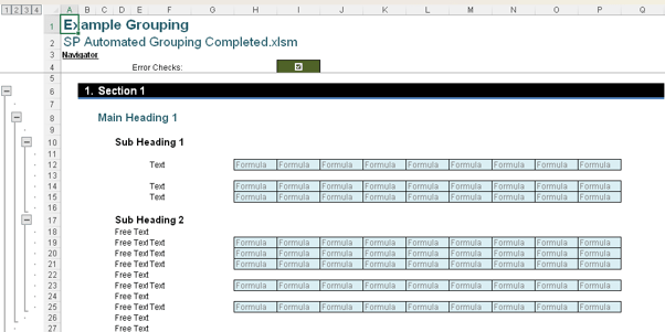
This ensures rows are ungrouped correctly, even if users accidentally enter free text in column D. viz

Similarly, you can write the same If condition for column C:

For Each rng In Range("C" & firstRow & ":C" & lastRow)
    If Not IsEmpty(rng.Value) And (rng.Style = "Heading 2 Text" Or rng.Style = "Heading 2 Number") Then
        rng.Rows.Ungroup
        rng.Rows.Ungroup
        rng.Offset(-1, 0).Rows.Ungroup
        rng.Offset(1, 0).Rows.Ungroup
    End If
Next

Finally, we can consider column B:

For Each rng In Range("B" & firstRow & ":B" & lastRow)
    If Not IsEmpty(rng.Value) And (rng.Style = "Heading 1 Text" Or rng.Style = "Heading 1 Number") Then
        On Error Resume Next
        rng.Offset(-1, 0).Rows.Ungroup
        rng.Offset(-1, 0).Rows.Ungroup
        rng.Offset(-2, 0).Rows.Ungroup
        rng.Offset(1, 0).Rows.Ungroup
        rng.Rows.Ungroup
        rng.Rows.Ungroup
        rng.Rows.Ungroup
        On Error GoTo 0
    End If
Next

Adding the style check helps the code identify the correct heading level, rather than simply detecting whether columns B, C or D contain a value.  This version confirms that the cell contains both a value and an appropriate heading style.  Here is the full code for grouping the headings by style:

Sub rowGroupingwithStyle()

Dim rng As Range
Dim firstRow, lastRow As Integer

'Expand all grouped rows (if any)
ActiveSheet.Outline.ShowLevels RowLevels:=8, ColumnLevels:=8

'Define first row and last row
firstRow = ActiveSheet.UsedRange.Row + 5
lastRow = ActiveSheet.UsedRange.Rows(ActiveSheet.UsedRange.Rows.Count).Row

'Unhide all rows (if any) and clear the outline
Rows(firstRow & ":" & lastRow).EntireRow.Hidden = False
Rows(firstRow & ":" & lastRow).ClearOutline
On Error Resume Next

'Group the rows from first row to last row to grouping level 4
Rows(firstRow & ":" & lastRow).Rows.Group
Rows(firstRow & ":" & lastRow).Rows.Group
Rows(firstRow & ":" & lastRow).Rows.Group

'Ungroup each row in column D that is not empty
For Each rng In Range("D" & firstRow & ":D" & lastRow)
    If Not IsEmpty(rng.Value) And (rng.Style = "Heading 3 Text" Or rng.Style = "Heading 3 Number") Then
        rng.Rows.Ungroup
    End If
Next

'Loop through each range in column C that is not empty
'If the range is not empty, ungroup current row twice
'If the range is not empty, ungroup the rows above and below the current row
For Each rng In Range("C" & firstRow & ":C" & lastRow)
    If Not IsEmpty(rng.Value) And (rng.Style = "Heading 2 Text" Or rng.Style = "Heading 2 Number") Then
        rng.Rows.Ungroup
        rng.Rows.Ungroup
        rng.Offset(-1, 0).Rows.Ungroup
        rng.Offset(1, 0).Rows.Ungroup
    End If
Next

'Loop through each range in column B that is not empty
'If the range is not empty, ungroup the row below current row twice
'If the range is not empty, ungroup the row above current row
'If the range is not empty, ungroup current row three times
For Each rng In Range("B" & firstRow & ":B" & lastRow)
    If Not IsEmpty(rng.Value) And (rng.Style = "Heading 1 Text" Or rng.Style = "Heading 1 Number") Then
        On Error Resume Next
        rng.Offset(-1, 0).Rows.Ungroup
        rng.Offset(-1, 0).Rows.Ungroup
        rng.Offset(-2, 0).Rows.Ungroup
        rng.Offset(1, 0).Rows.Ungroup
        rng.Rows.Ungroup
        rng.Rows.Ungroup
        rng.Rows.Ungroup
        On Error GoTo 0
    End If
Next

ActiveSheet.Outline.SummaryRow = xlAbove

'Go back to range A1
Range("A1").Select

End Sub