Broadcasting: Making Sense of Arrays

Most Excel users happily build formulas while unaware that a technique known as broadcasting underpins many of their calculations. The goal of this post is to explain what broadcasting is and to demonstrate how you can use it intentionally.

Basic array behaviour

Let’s start at the beginning.

An array is simply a collection of values. For example, in Excel, the following is an array.

{1,2,3;4,5,6;7,8,9}

The comma is the column separator, and the semicolon is the row separator. These are the standard UK characters for arrays in Excel; your region settings may use different characters.

Just by looking at the array, it may be difficult to see what’s happening, so I have visualized it.

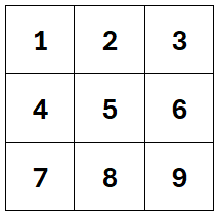
As you can see, this is just a grid with rows and columns. Ranges in Excel are also a grid with rows and columns; therefore, Excel often converts between ranges and arrays for calculation.

When we have individual values, we can easily perform calculations:

1 + 1 = 2

But what happens when the values are not individual values, but arrays?

{1,2,3;4,5,6;7,8,9} + {1,2,3;4,5,6;7,8,9}

Here is the visual representation of this calculation.

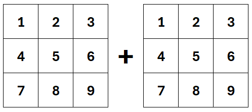
Excel performs the calculation by matching values based on their position within each array.

• For row 1 column 1: 1 + 1 = 2
• For row 1 column 2: 2 + 2 = 4
• For row 1 column 3: 3 + 3 = 6
• …
• For row 3 column 3: 9 + 9 = 18

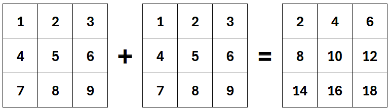
The output is another array.

{1,2,3;4,5,6;7,8,9} + {1,2,3;4,5,6;7,8,9}
= {2,4,6;8,10,12;14,16,18}

The visual representation of this is:

Once we understand this basic array behaviour, we can start looking at broadcasting.

Broadcasting

Broadcasting occurs when Excel performs calculation with arrays of different sizes.

For example, what should happen in this scenario?

{1,2,3;4,5,6;7,8,9} + {1}

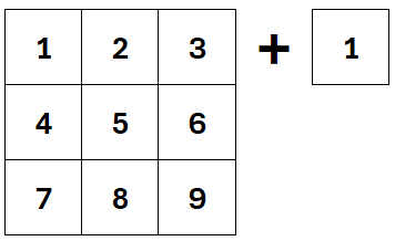
The arrays are different sizes.

The first array is 3 x 3, the second array is 1 x 1. To perform this calculation, broadcasting occurs.

Excel expands the smaller array to match the shape of the larger array. This then allows the calculation to occur by position.

The calculation becomes:

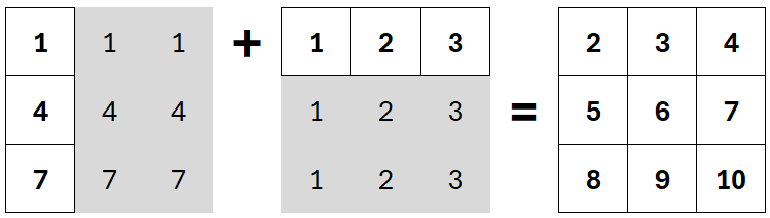
{1,2,3;4,5,6;7,8,9} + {1,1,1;1,1,1;1,1,1}
= {2,3,4;5,6,7;8,9,10}

The visual representation of this is:

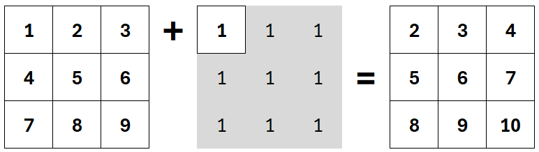
The values in the grey area have been broadcast. They don’t exist anywhere; they are generated in the background solely to perform the calculation.

That is a single-value example. But we’re not restricted to single values.

In the example below, a single column is broadcast to enable the position calculation to occur. 

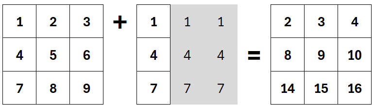
Once again, the grey area is the broadcast values that we don’t see visually.

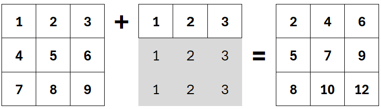
We get the same treatment with rows.

The examples above are based on arrays containing a single row and/or a single column. Technically, broadcasting happens with arrays of any size. However, if there are multiple rows and columns, Excel doesn’t know which values to broadcast, so it generates #N/A for the missing values.

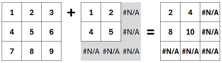
This is not particularly useful. Therefore, we tend to use arrays which have only one row or column.

As our final example for this section, what happens when there is a single row and a single column?

1. The first array expands to the size of the second array.
2. The second array expands to the size of the first array. 
3. The calculation occurs based on position.

The output looks like this:

This applies the same broadcasting principles, but it might take a little thought to get your head around it.

Applying it to Excel

When we apply the broadcasting concept in Excel, a formula might look like this:

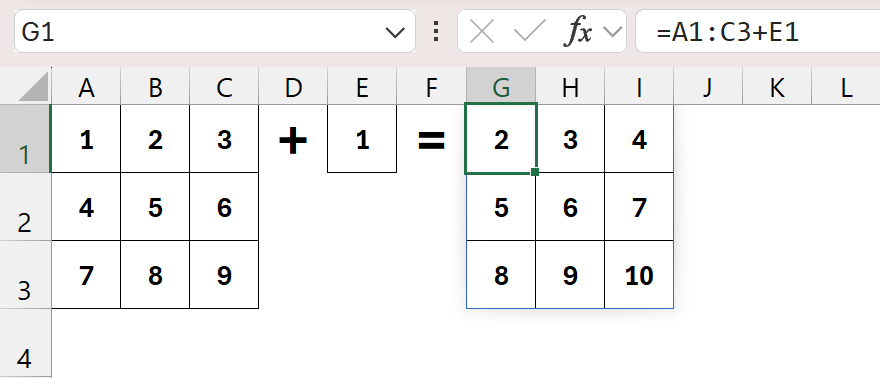
The formula in cell G1 is:

=A1:C3+E1

Excel changes the ranges into arrays, broadcasts any values, performs the calculation based on position, and returns the array to the grid.

We don’t see the broadcast values; it happens in the background.

You might be wondering why there are no $ signs.

It’s a common question. You might have expected the formula in G1 to be:

=$A$1:$C$3+$E$1

Absolute references are only required when a formula is copied to another location. In this example, the formula exists only in cell G1. 

Excel’s formula creates an array of multiple values and returns them to the grid in a “spill” range.

The formula has not been dragged or moved. Therefore, the $ is not required.

Use broadcasting intentionally?

Now we know what broadcasting is, we can use it intentionally with calculations.

Let’s take a look at some common examples.

Financial modelling

This is a simple financial modelling example.

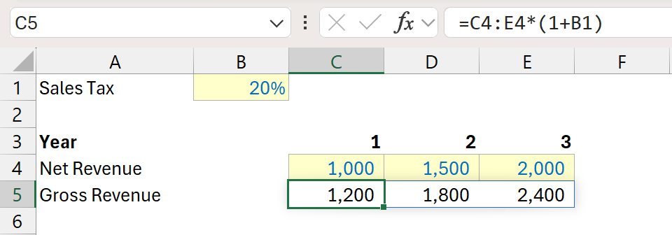
Cell C5 contains the formula:

=C4:G4*(1+B1)

The 1.2 created by 1+B1 is broadcast, the calculation occurs by position, and Excel returns the result.

We could represent the broadcasting as follows:

SUM / SUMPRODUCT logic

Using SUMPRODUCT for two-dimensional lookups is a scenario many Excel users will be familiar with.

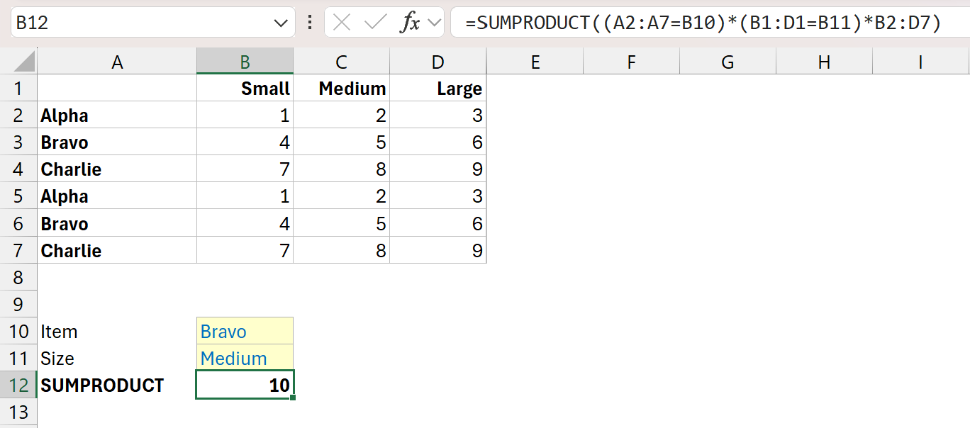
The formula in cell B12 is:

=SUMPRODUCT((A2:A7=B10)*(B1:D1=B11)*B2:D7)

Inside SUMPRODUCT, there are 3 arrays of different sizes multiplied together.

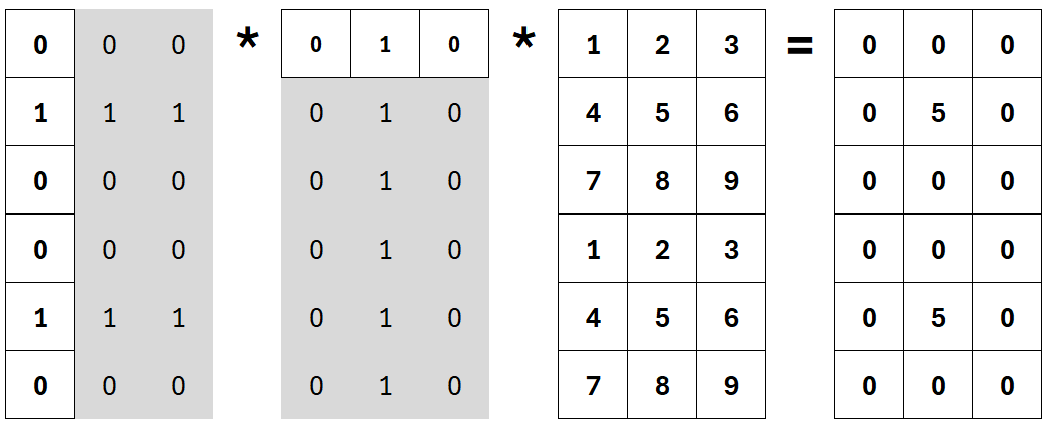
In the table above, TRUE/FALSE are converted to 1 and 0 for convenience of display.

The result of the 3-array calculation is passed into SUMPRODUCT to calculate the single result.

=SUMPRODUCT({0,0,0;0,5,0;0,0,0;0,0,0;0,5,0;0,0,0})

Inside FILTER

In this example, we’re looking at the include argument of the FILTER function.

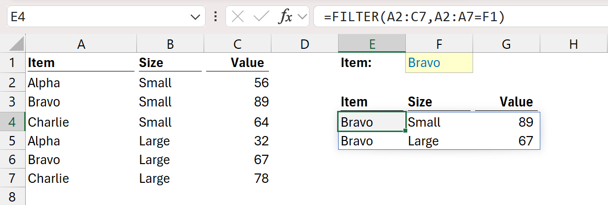
The formula in cell E4 is:

=FILTER(A2:C7,A2:A7=F1)

This formula returns the rows from A2:C7 where A2:A7 is equal to F1.

In the second argument, F1 is broadcast for each row in A2:A7 to create an array of TRUE and FALSE values.

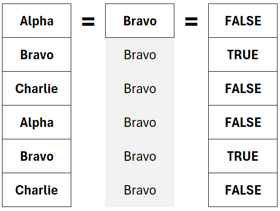
This creates an array which is used inside FILTER to return the relevant values.

=FILTER(A2:C7,{FALSE;TRUE;FALSE;FALSE;TRUE;FALSE})

Replacing IF with logic

Using boolean logic we can replace the IF function.

In the screenshot below, we want to return the value if it is greater than or equal to 75; otherwise, return 0. 

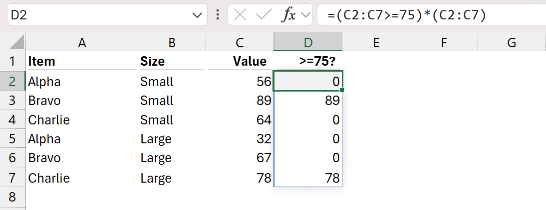
The formula in cell D2 is:

=(C2:C7>=75)*(C2:C7)

This formula can be visualized as follows:

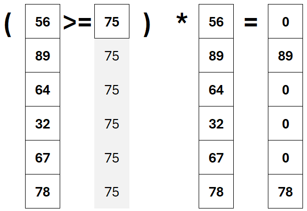
In this example, there are 3 arrays; the 75 is broadcast to enable calculation to occur based on position.

Conclusion

Broadcasting is one of Excel's fundamental behaviours. Whenever Excel performs calculations between arrays of different sizes, it automatically expands the smaller array so it can calculate based on position.

Most of the time, broadcasting happens invisibly in the background. However, once you understand how it works, many Excel formulas become much easier to understand and build.