Excel speed up productivity tricks - formulas

Instead of typing in formulas, try this:

1. Aggregations on bottom right: You have probably noticed that when you select some cells, Excel shows a SUM on the bottom right. Here are some pro tips:
   
   1. If you right click the SUM, you can edit which aggregations appear. I personally tick them all, because well - why not.
   2. If you left click a cell, that will copy the number, which can be pasted into another cell, a WhatsApp message to mum, anywhere. It turns darker when you hover over and can copy as shown.

2. Autosum: If you’re tired of typing in the whole SUM formula, click the Sigma icon (Σ) on the top right to sum all numbers above or to the left. Pro tips:
   1. Select the cells and press Alt = together to get the same outcome.
   2. Select an entire table and Alt = will put sums in all the rows and all columns
3. Use Copilot or other AI to convert a description into a formula: Type the right prompt, copy the outcome, then paste into your formula bar and then it works - hopefully, if AI didn’t hallucinate.
4. Copilot suggest formulas: Copilot premium subscribers can benefit from suggestions which pop up on pressing =, this depends on the cells around it. It’s a useful feature, but not always predictable when it will pop up.
5. Function creation wizard: Click Formulas tab > Insert function to launch this guide
6. Formulas tab > Recently used functions: This should be useful but it’s an outright lie; my list contains the SIN function that I don’t think I’ve ever even used.
7. PivotTables are easier to aggregate by category than formulas: If you are a big SUMIFS person who finds it tedious to write many formulas, try PivotTables. It’s a whole world with its own productivity speed up tricks article that I wrote a few months back. This video has an introduction:

Write formulas more efficiently

8. Function autocomplete from any letter: Type a few letters anywhere and Excel will give options, note that this recently got upgraded so you can type anywhere in the word e.g. type “=kup” and Excel will give options for VLOOKUP, XLOOKUP, LOOKUP etc. 
9. Press Tab to lock in a function: When you have the function you want selected in blue, type the Tab key or double click to lock it in. Note, even though Excel typically shows function names in UPPERCASE, using lowercase works too.
10. Ctrl Shift U expands or contracts the formula bar: If you need more room mid formula, this can be handy.
11. Alt Enter starts a new line in a formula: To neaten up a complex formula, create a new line with Alt Enter. Neither new lines nor spaces in formulas have any consequence on the formulas themselves.

Get output formulas to autocomplete when new rows are added

12. Formulas can now reference an array: E.g. instead of computing a single cell =A1+B1 in C1 then filling down until A30, you can now use =A1:A30+B1:B30 in cell C1 and the outcome result would be in cells C1:C30 with a blue outline around them. This is called a Dynamic Array or a Spill Array and got released in 2020. Pro tips:
1. If you ever see a =SPILL# error, this is usually because an array is trying to spill into cells occupied by existing data.
2. You can reference an entire array using # notation, e.g. =C1# returns the entire Spill Array starting in cell C1. = SUM(C1#) will add all the cells in that array.
3. Excel released a slew of new functions with this new Dynamic Array capability, I cover 24 in my video here:

13. =TRIMRANGE or . notation – from 2025: Let’s say you want to pre-populate an output column, but only have the output show up when the data is filled in. e.g. the formula “=IF(A1=”Read”, “Book”, “Movie”) gets dragged down for new rows of data to A10, but if some cells at the bottom are empty or now, it will return “Movie”, which seems wrong. Instead wrap it in =TRIMRANGE and use an array, type =TRIMRANGE(IF(A1:A10=”Read”, “Book”, “Movie)). Note, you can also use . notation, so = IF(A1.:.A10=”Read”, “Book”, “Movie) returns the same output.

Type once then reuse

1. Name manager: If you reuse a cell or a range often in a formula, you may want to name it, e.g. if B2 contains the USD to Euro exchange rate, you can go to Formulas tab > Name Manager and name the cell B2 as “ExchangeRate”. After that, =E5*ExchangeRate or =H4*ExchangeRate will convert across currencies.
2. Create your own custom functions with  LAMBDA: How many names are in this list: Frank, Donna, Frank, Donna, Lisa. Well Excel has no way of returning 3 for a unique count. Google Sheets has =COUNTUNIQUE but not Excel. You can though create that function using the name manager, a function called LAMBDA and an overly complicated unintuitive method. The function =COUNTA can count the cells with data in a range, and =UNIQUE can create a unique list, its actually one of those nifty “Dynamic Array” functions mentioned above. =COUNTA(UNIQUE(Cells)) will therefore return a count of unique cells, but you can even define a new function called, say, UNIQUECOUNT to do just that. Enter the formula in a cell =LAMBDA(Cells,COUNTA(UNIQUE(Cells)). The output is unhelpfully an error which says #CALC! but, if you copy that formula, then go to Formula tab > Name Manager and click New, you can paste that into “Refers to” and give it a name as shown here:

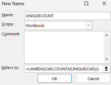
LAMBDAs are stored at the workbook level; there isn’t currently a way to hold them across all your Excel files. The video below has more information on LAMDBDA

3. LET: Define a part of a formula and reuse it later. Let’s say you want a sum but only if numbers to always return a number above 5, otherwise you’d add 5. The full formula looks like this: =IF(SUM(A1:A20)>5, SUM(A1:A20),5+ SUM(A1:A20)). Instead of repeating SUM(A1:A20), thrice though, you could instead let the name AddCells refer to the sum of A1:A20, so an equivalent using the LET function introduced this decade could be: =LET(AddCells, SUM(A1:A20),IF(AddCells>5,AddCells,5+AddCells))

Filling down is slow, try these tricks instead

4. Select the cell with the formula, then double click the bottom right instead of dragging down.
5. Select the cells below the formula you’d like to fill down together with the cell containing your formula and click Ctrl D, note to fill right its Ctrl R).
6. As you’re typing the formula, select all the cells where you want the formula to be, and instead or pressing enter to lock it in, press Ctrl Enter.
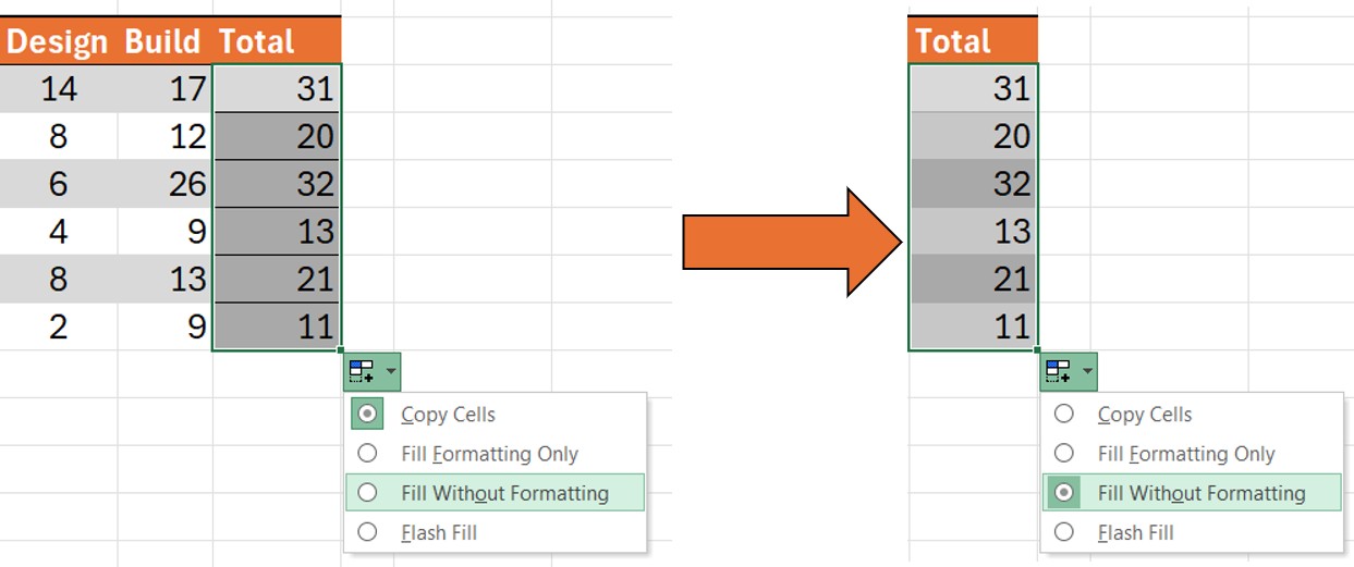
7. Filling down formulas often breaks formats as it copies the cell formats from the topmost cell, but this is very easy to disable, click the pop-up box then choose “Fill Without Formatting”.

That wraps up this third edition of speed up productivity tricks but check back in for another one in the coming months.