Any Interest in Mortgage Schedules?

For chartered accountants, this is not simply an Excel exercise.  A dependable debt schedule supports interest expense, current and non-current debt classification, cash flow forecasting, covenant analysis and the reconciliation of financing balances.  If the schedule is wrong, several parts of the financial statements may be wrong with it.

In this article, I shall build a monthly mortgage schedule using formulae only.  I will use the attached Excel file as my example

Setting the Scene

I will use the following assumptions:

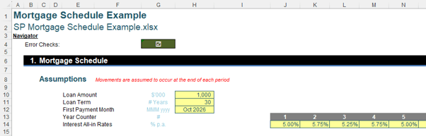
The loan amount is $1,000,000 entered as 1,000 because the model is presented in thousands.  The loan runs for 30 years, with the first payment in October 2026.

Rather than assuming one interest rate throughout, cells J13:AM14 with a named range Interest contain the all-in interest rate for each loan year.  This allows the payment to adjust when the applicable rate changes.

Building the Schedule

First, I need to convert the loan term into months in cell H19 using the formula below:

= Loan_Term*Months_in_Year

The schedule itself contains 360 rows, allowing for loans of up to 30 years.  Only the rows required by the selected loan term will be active.

That flexibility matters in practice.  It allows you to use the same controlled calculation for budgeting, refinancing analysis and reporting, rather than maintaining several near-identical schedules that may cease to agree.

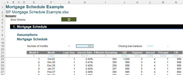
The first calculation of the schedule is ‘Month #’ in cell E23:

=N(E22)+1

The N function is used to return the number value of a cell reference.  If the reference contains text, the function will return zero [0].  If it is a number, that number will be returned.  This starts the schedule at Month 1 and increases by one as the formula is copied down.

Next, I need the actual payment Month:

=EDATE(First_Payment,$E23-1)

EDATE moves forward from the first payment month in H12.  Month 1 is therefore October 2026, Month 2 is November 2026 and so on.

The ‘Loan Year’ in G23 is then:

=ROUNDUP(E23/Months_in_Year,0)

Months 1 to 12 belong to Loan Year 1, Months 13 to 24 belong to Loan Year 2, etc.  This loan year is used to select the appropriate interest rate.

Cell H23 calculates the ‘Interest Rate’ for the month:

=LOOKUP(G23,Interest)*DAY(EOMONTH(F23,0))/Days_in_Year

The LOOKUP returns the annual all-in rate applying to the relevant loan year in cell G23.

The second part converts that annual rate into a monthly rate using the ratio of actual number of days in the month over total days in a year specified by Days_in_Year.  EOMONTH identifies the month-end date of the corresponding Month in F23 and DAY returns the number of days in that month.

This day-sensitive approach is relevant where interest accruals must reconcile to the general ledger.  February is not March, leap years occur and a simple annual rate divided by 12 may not reproduce the amount charged by a lender.

Next, I calculate the ‘# Months Remaining’ by taking the number of months in H19 less the corresponding ‘Month #’ in cell E23 and plus one [1].

=MAX($H$19-E23+1,0)

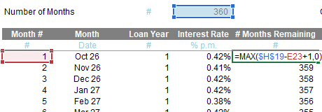
At Month 1, there are 360 months remaining; at Month 2, there are 359.  The MAX prevents the result becoming negative after the loan term has finished, which is useful given that the calculation area extends to 360 rows.

The opening balance O/B in J23 is:

=IF($E23=1,Loan_Amount,N22)

For Month 1, the opening balance is the original loan amount.  Thereafter, each month’s opening balance is simply the previous month’s closing balance.

Now comes the mortgage Payment:

=IF(I23=0,0,-PMT(H23,I23,J23))

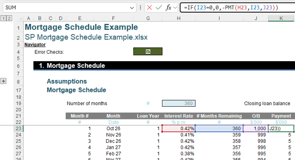
PMT calculates the payment required based on three [3] things: the applicable monthly interest rate, the number of months remaining and the opening loan balance.  The minus sign converts Excel’s negative cashflow result into a positive payment for presentation purposes.

An important point here is that the payment is recalculated each month.  If the all-in interest rate changes between loan years, the payment adjusts based on the new rate, outstanding balance and remaining term.

For accountants, this also makes the schedule useful for forecasting debt service and assessing liquidity or covenant headroom.  A rate change affects more than interest expense: it may alter the cash payment as well.

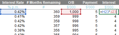
Once the payment is known, Interest in L23 is simply the monthly interest rate multiplied by the opening balance:

=H23*J23

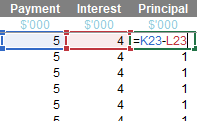
Principal in M23 is then the difference between the monthly Payment and Interest paid:

Finally, the closing balance C/B in N23 is:

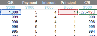
The closing balance becomes the opening balance for the following month and the process repeats.

Together, the opening balance, interest, principal and closing balance form a compact debt roll-forward.  That makes the schedule easier to audit and gives the preparer a clear bridge from the lender statement to the ledger and financial statement disclosures.

Checking the Loan Balance

One final calculation in cell M19 shows the closing balance at the end of the contractual loan term: =INDEX(N23:N382,H19)

The mortgage schedule contains 360 possible monthly balances, but ‘Number of Months’ in cell H19 tells us which one represents the actual end of the loan.

For a fully amortising mortgage, I would expect this balance to be zero [0], subject to normal Excel precision and rounding.  If it isn’t, there is something worth investigating.

This is a useful control rather than merely a pleasing answer.  The maturity balance should reconcile, and accountants should also sense-check total payments, interest expense and the split between amounts due within and after 12 months.

Word to the Wise

There is nothing particularly exotic about a mortgage schedule.  The trick is making each calculation do one job and making the relationships between them easy to follow.  That transparency matters when the model is reviewed, handed over or used to support an accounting judgement.

Each month starts with an opening balance.  Interest is calculated, the payment is split between interest and principal, and principal reduces the loan to its closing balance.  Then, we do it all again next month.  In accounting terms, it is a disciplined roll-forward: opening balance, movements and closing balance.

The same 360-row schedule can accommodate different loan amounts, terms, payment dates and annual interest rates without rewriting a single formula.  That consistency reduces manual intervention and makes changes easier to explain and review.

Sometimes, good financial modelling really is just paying attention to the details.  We already know the importance of reconciliations and controls; a well-built mortgage schedule simply puts those disciplines to work in Excel.