Number formats again – making a dash for it

Introduction

In part one of the series, we emphasised how much difference a suitable number format could make to the clarity and impact of a financial report, and we saw how we could create a very specific number format using the custom number format functionality, before considering in part 2 how to make our custom number format easy to apply. We will finish the series with a brief look at some less obvious issues arising from the use of custom number formats and some more advanced capabilities.

£’000

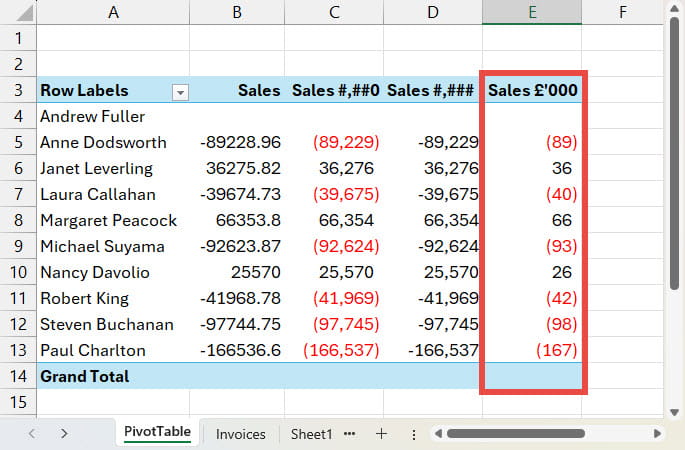
We’ve seen how to display a number as round pounds, but it’s worth considering how we would round the display to other units, such as thousands. In fact, it’s relatively simple. We can add a comma at the end of each of our blocks of placeholder characters:

Displayed to pounds: #,##0_);[Red](#,##0);-?

Displayed to thousands of pounds: #,##0,_);[Red](#,##0,);-?

We have added a column to our PivotTable to demonstrate this:

We could even extend this to millions by adding a second comma:

#,##0,,_);[Red](#,##0,,);-?

This gives us the slightly concerning result shown below:

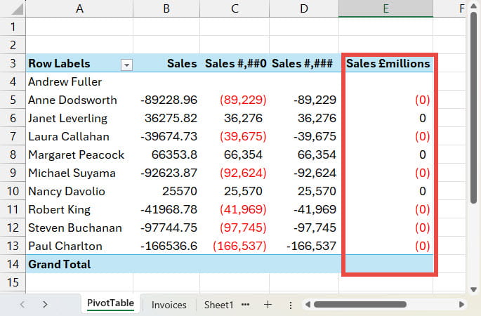
Although all our figures are below 500,000, so we should expect to see values representing zero, we deliberately set our custom number format up to replace zeros with dashes. The reason is that, although the formatting ‘rounds’ the display of the values to zero, the values themselves have not been rounded so are not zero and the third, zero, section of our number format is only used for values that are ‘really’ zero. In many situations, the easiest solution is to round our values to the same number of digits as our display. For example, for millions we would set the second argument of our ROUND() function to -6 being six digits to the left of the decimal point:

=ROUND(E5,-6)

Rounding the values in this way will sort the formatting out but does need to be approached with care since rounding obviously reduces the precision of the values held, affecting any calculations based on the rounded values.

Negative conditional success

Given the concerns about actually rounding the values themselves, there is a tempting capability of custom number formats that looks as though it should apply dashes successfully, even when the display causes non-zero values to be displayed as zero.

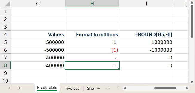
Although the first two sections of the number format are usually used for positive and negative numbers respectively, they can also be used to apply conditions. Section 1 holds the condition for the largest numbers, section 2 for the smallest numbers leaving section 3 for anything that fails the conditions in the first two sections. You might expect the example below to solve our zero/non-zero issue. Any number above 500,000 will have our ‘positive’ format applied and any number equal to or below -500,000 will have our ‘negative’ number applied. This should leave the third section to format any number between -500,000 and 500,000 as a dash:

[>=500000]#,##0,,_);[Red][<-500000](#,##0,,);-_)

However, this is not quite what happens. Negative values above -500000 are shown as minus dash rather than just as a dash:

I’ve not been able to come up with a simple solution to use just custom number formatting to display dashes successfully when numbers aren’t actually rounded. If you know a way, pleases let us know!

Another thing

It’s also worth noting that if a condition is not specified in one of the first two sections, the default condition of positive for the first section and negative for the second section will apply. Also, note that the conditions are evaluated from left to right, so:

[Red][>100]#,##0;[Blue][>500]#,##0;[Green]#,##0

would show all numbers above 100, including those above 500, in red.

Additional resources

The Power BI based ICAEW Excel archive portal includes several detailed articles on number formatting. Select the ‘Formatting’ keyword to see a list:

The 'Open in full-screen mode' icon in the bottom right-hand corner of the embedded report should show the contents at a more readable size with the Escape key returning you to the post.