Returning a subset of data with just one formula

For example, imagine we have the following larger table:

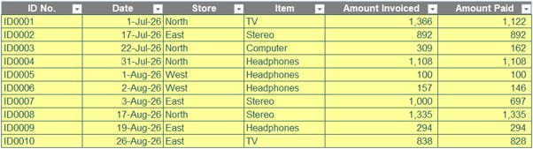
OK, so it’s not the world’s largest table – but bear with me, the concept remains intact!

The aim was that when values were typed into the ID No. assumption cells below, the table would populate using just one formula typed into the top left-hand corner of the range and would thus populate the whole range, viz.

If fields (columns) or ID values (records) were to change, I would want the formula to automatically recalculate:

Where values cannot be found, the results should have returned blank cells as pictured above.

My example Excel file shows how I approached the problem. Of course, XLOOKUP, INDEX MATCH, VLOOKUP and many other alternatives could be used to generate the result by copying into one cell and then extending the formulae across columns and down rows accordingly – but I just wanted to type one formula into one cell and watch the whole thing populate.

This is what I came up with:

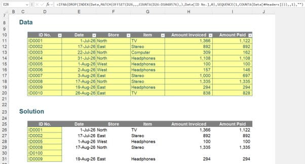
Please note the cell references in order to understand the rest of our solution.

For those who don’t have microscopes to hand, the formula is given by:

=IFNA(DROP(INDEX(Data,
MATCH(OFFSET(D26,,,COUNTA(D26:D1048576),),Data[ID No.],0),
SEQUENCE(1,COUNTA(Data[#Headers]))),,1),"")

First, I will use the INDEX function. This needs a version of Excel that supports dynamic arrays. This is necessary for the results to “spill”.

Essentially,

INDEX(array, row_number, [column_number])

returns a value or the reference to a value from within a table or range (list).

For example,

INDEX({7,8,9,10,11,12},3)

returns the third item in the list {7,8,9,10,11,12}, ie, 9.

This could have been a range: INDEX(A1:A10,5) gives the value in cell A5, etc.

INDEX can work in two dimensions as well (hence the column_number reference). Consider the following example:

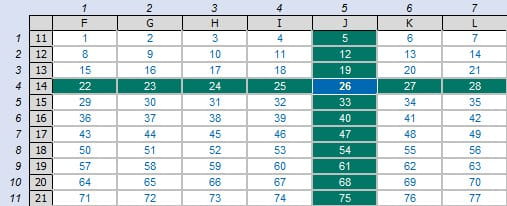
INDEX(F11:L21,4,5) returns the value in the fourth row, fifth column of the table array F11:L21 (clearly 26 in the above illustration). This is how I am using it here.

For the array argument, I refer to the original table labelled Data. For the row argument, I will use the following formula:

MATCH(OFFSET(D26,,,COUNTA(D26:D1048576),),Data[ID No.],0)

In this formula

MATCH(lookup_value, lookup_vector, [match_type])

returns the relative position of an item in an array that (approximately) matches a specified value. It is not case sensitive. The MATCH function here returns a row number by matching these two components:

• OFFSET(D26,,,COUNTA(D26:D1048576),) is the range for the IDs whose data you want to return (the input ID No. values) – I will explain this better in a moment.
• Data[ID No.] is the field of the IDs in the original table, Data.

You should note that the optional match_type is zero [0] meaning it will return the first exact match.

So what of this?

OFFSET(D26,,,COUNTA(D26:D1048576),)

This uses the OFFSET function, which has the following syntax:

OFFSET(reference, rows, columns, [height], [width])

Cell D26 is the starting point (the first ID No.). The reference is not displaced any rows or columns, but the height is specified:

COUNTA(D26:D1048576)

This counts the number of non-blank cells in the range D26:D1048576, the latter being the final cell in the column. If six values for ID No. are typed in, this will have a value of six; if there are seven, it will be seven, and so on. It tells MATCH how many rows it must consider – assuming all cells thereafter are blank (else change the reference range).

The INDEX function will use the height to return the appropriate number of rows of data, in this case, the rows will spill. For the third argument of the INDEX function, column, instead of using another MATCH formula (we know the order of columns), I will “simply” use the following:

SEQUENCE(1,COUNTA(Data[#Headers]))

where:

• Data[#Headers] is the range of headers in the provided data table, Data.
• COUNTA counts the number of headers in the provided data table, Data.
• SEQUENCE spills out column counters based upon the number of headers in the provided data table, Data. In essence, it propagates the formula across columns.  With a syntax of SEQUENCE(rows, [columns], [start], [step]), I need the range to spill over one [1] row, hence the COUNTA expression is used to drive the number of columns (the last two arguments are unnecessary).

In some cases, if there is no match between any proposed IDs and the IDs in the original provided data table, this formula will return an error. To ensure all errors are replaced with blank text (""), I will use the INDEX function nested within an IFNA function.

With both the row and column parameters defined and errors handled, the correct data can be returned. However, there will be an extra ID column produced, as written. I can remove this with the use of the DROP function

DROP(array, rows, [columns])

which can “drop” the first column:

• The array argument is the INDEX calculation above.
• The rows argument is zero [0].
• The columns argument is one [1], thus removing the first column.

With that, I arrive at the final solution:

=IFNA(DROP(INDEX(Data,
MATCH(OFFSET(D26,,,COUNTA(D26:D1048576),),Data[ID No.],0),
SEQUENCE(1,COUNTA(Data[#Headers]))),,1),"")