Searchable Data Validation

To access data validation, from any cell in Excel:

• on the Data tab of the Ribbon, go to the ‘Data Tools’ group and click the ‘Data Validation’ icon (ALT + A + V + V)
• alternatively, the old Excel 2003 and earlier keyboard shortcut ALT + D + L still works.

This brings up the following dialog box:

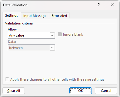
The default setting for all cells in Excel is to allow any value (pictured). This can be changed by changing the selection in the ‘Allow’ drop down box. It may be modified to any of the following:

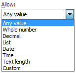
Most of these criteria do exactly what they say on the tin: by choosing ‘Decimal’, the input must be a number, whereas ‘Whole Number’ allows for integers only. However, making a selection from the ‘Allow’ drop down box is only the first part of the data validation process.

Once a selection has been made (for example, I will use ‘Whole Number’), the dialog box will change appearance, viz.

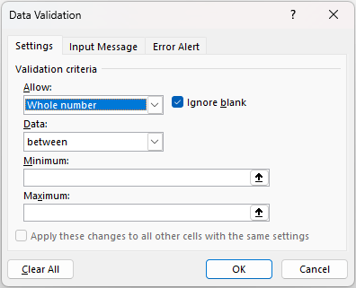
The ‘Ignore blank’ check box is no longer greyed out. This allows blank cells to be ‘valid’ regardless of the criteria selected. The remainder of the dialog box is governed by the ‘Data’ drop down box. There are various selections that may be made:

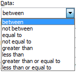
Depending upon the choice made, the box will prompt for values (e.g. Minimum and Maximum in the illustration above) which can be typed in, or else the values can refer to cell references directly or indirectly via range names.

Whole Number, Decimal, Date, Time and Text Length are all relatively straightforward, albeit very similar in nature. Custom allows you to customise your criterion / criteria using a formula, but the one I wish to concentrate on here is List, which allows you to select from a list.

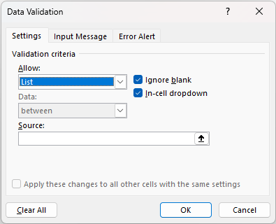
With ‘List’ selected, the dialog box prompts for a source for the list. Entries may be typed in, separated by a comma, but you can also use cell references or range names. For lists, I strongly recommend using the ‘In-cell dropdown’ which provides a dropdown list of valid entries once the cell has been selected.

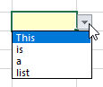
Data validated lists are great for forcing end users to choose from a predetermined selection, and prevent typos, accidental capitalisation and additional spaces from occurring – all of which can cause dependent formulae to fail, if left unnoticed.

Here, I want to create a searchable data validated drop down box using a method that would work in a perpetual licence version (e.g. Excel 2021) of Excel. You might argue this is already possible, but the results are unreliable is you are searching for a subset of a text string which is not the start of that string, e.g. “bin” in “Combination”.

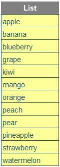
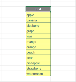
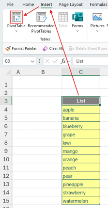
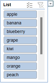
Consider the following list which I have given the name Data:

To start, select any cell on the list:

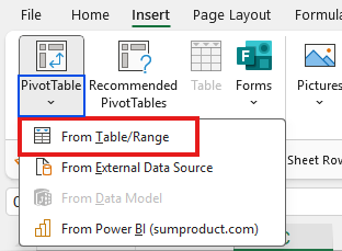
Go to the Ribbon, select ‘Insert’ tab and click the ‘PivotTable’ icon:

You may also click on the ‘PivotTable’ dropdown menu (blue) and then select ‘From Table/Range’ (red) to arrive at the same next step (not all options may appear in your version of Excel):

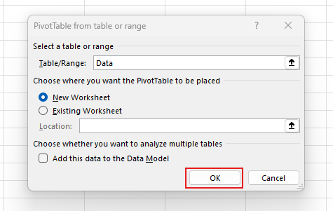
This will open the ‘PivotTable from table or range’ dialog. Click ‘OK’:

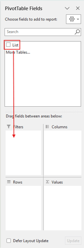
Focusing on the ‘PivotTable Fields’ pane, drag the List field down into the Filters area:

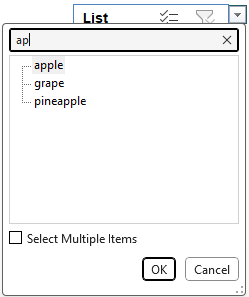
Then, apply proper formatting. It will create this, which is the successful completion of this month’s challenge:

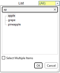
As an addition, you might want to use this trick to create a searchable box for a Slicer to enhance the end user experience:

The dropdown menu will open in front of the slicer:

Word to the wise

OK, so technically this isn’t a data validation list, but it is a data validated list. Only certain choices are permitted, which is actually you want. Sometimes, you have to think outside the hedgehog.