Excel Tip of the Week #386 - Power Pivot: RELATEDTABLE

The data, and the problem

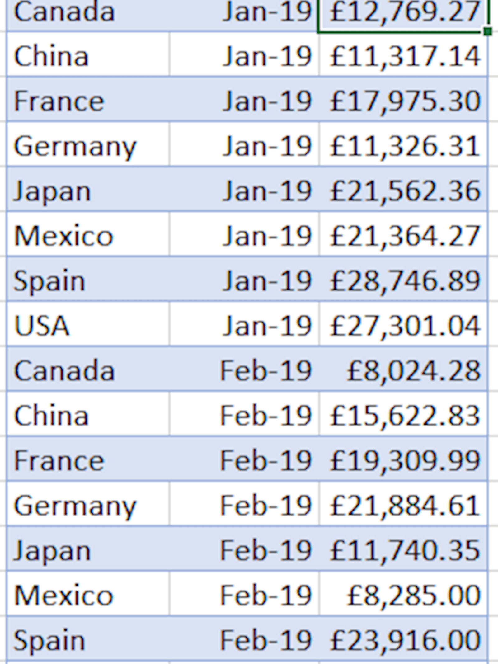
We have this table of sales over time:

We also have the sales reps who are active in each country:

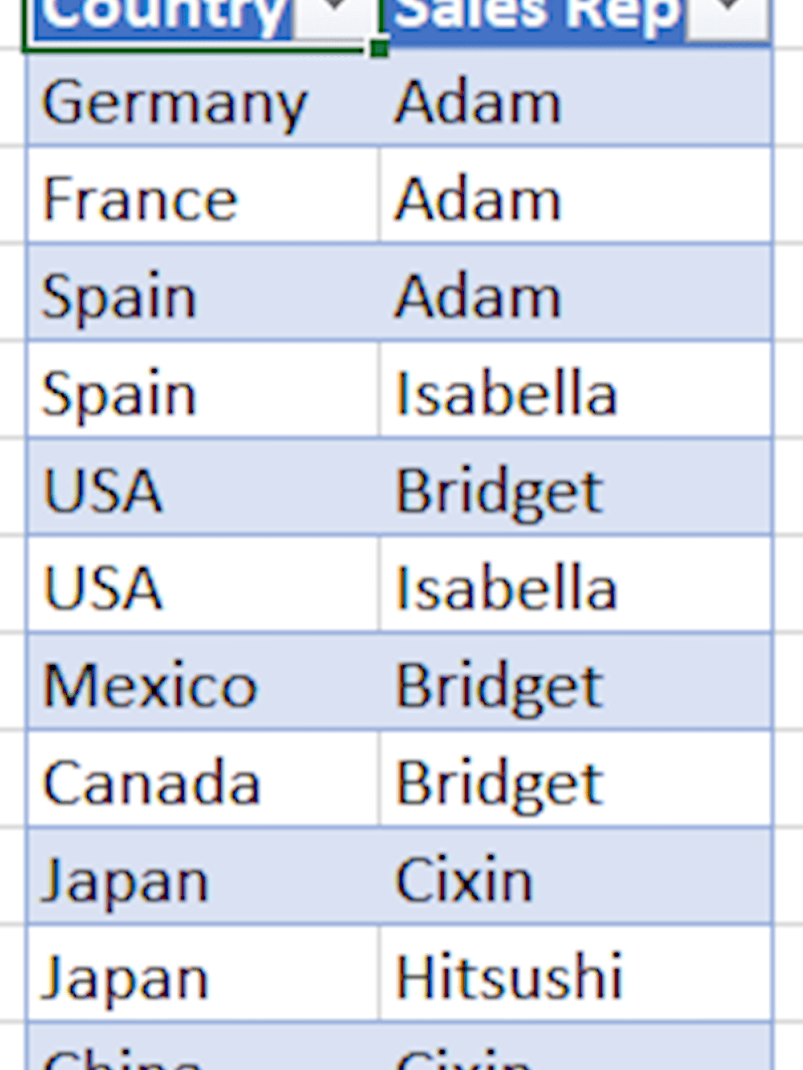
What we want is the total sales for each sales rep – including all the countries they are active in. Unlike previous situations we’ve examined, where we had categories which were expanded into further detail, here our two categories – sales reps and sales – both cover multiple countries, and neither ties to the country list uniquely – for example Adam and Isabella are both active in Spain. We can’t directly relate the two country fields as both contain duplicates, so there’s no way for Power Pivot to connect the two.

Solving the problem

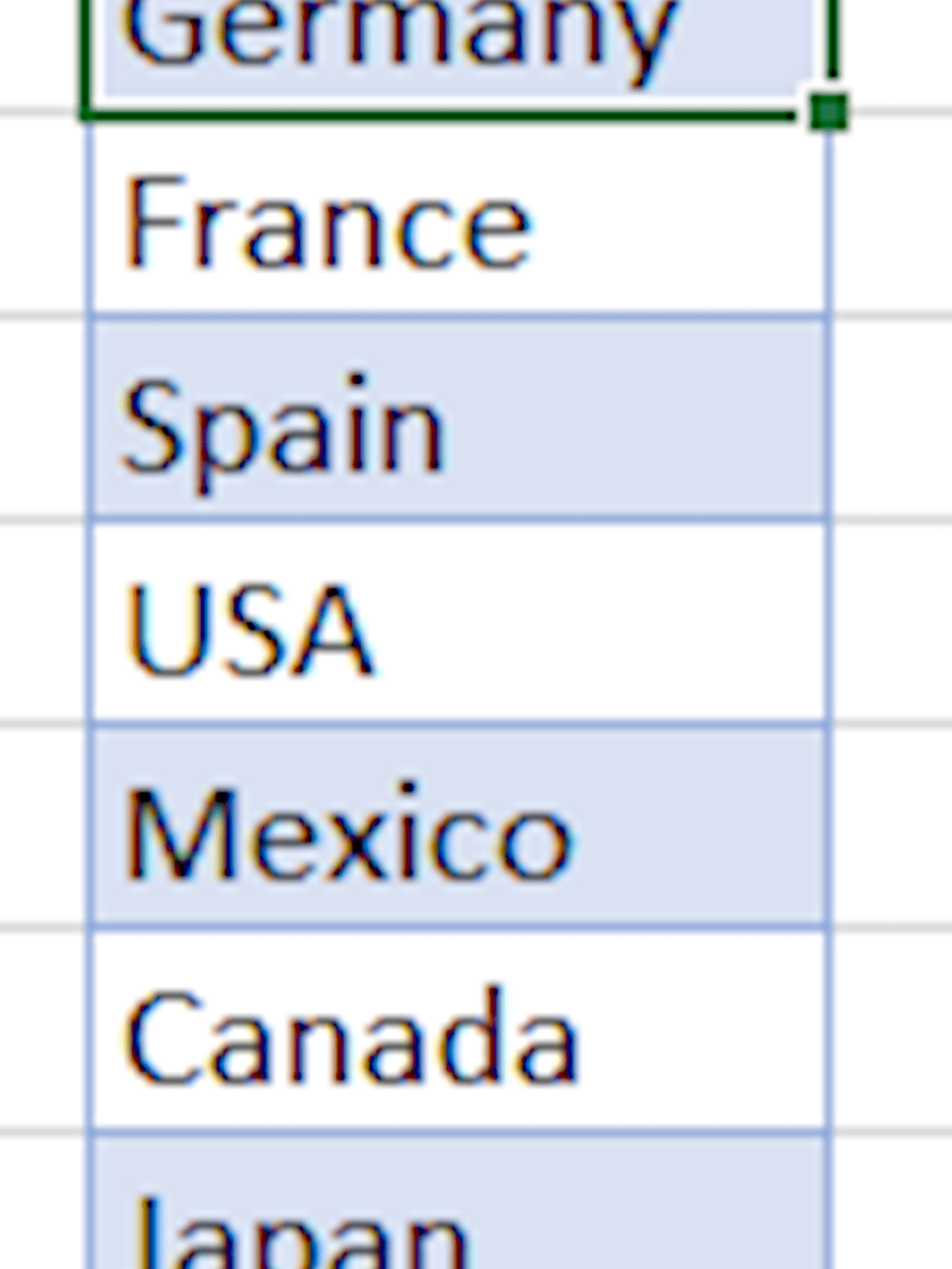
First, we will need to create a very simple country list table:

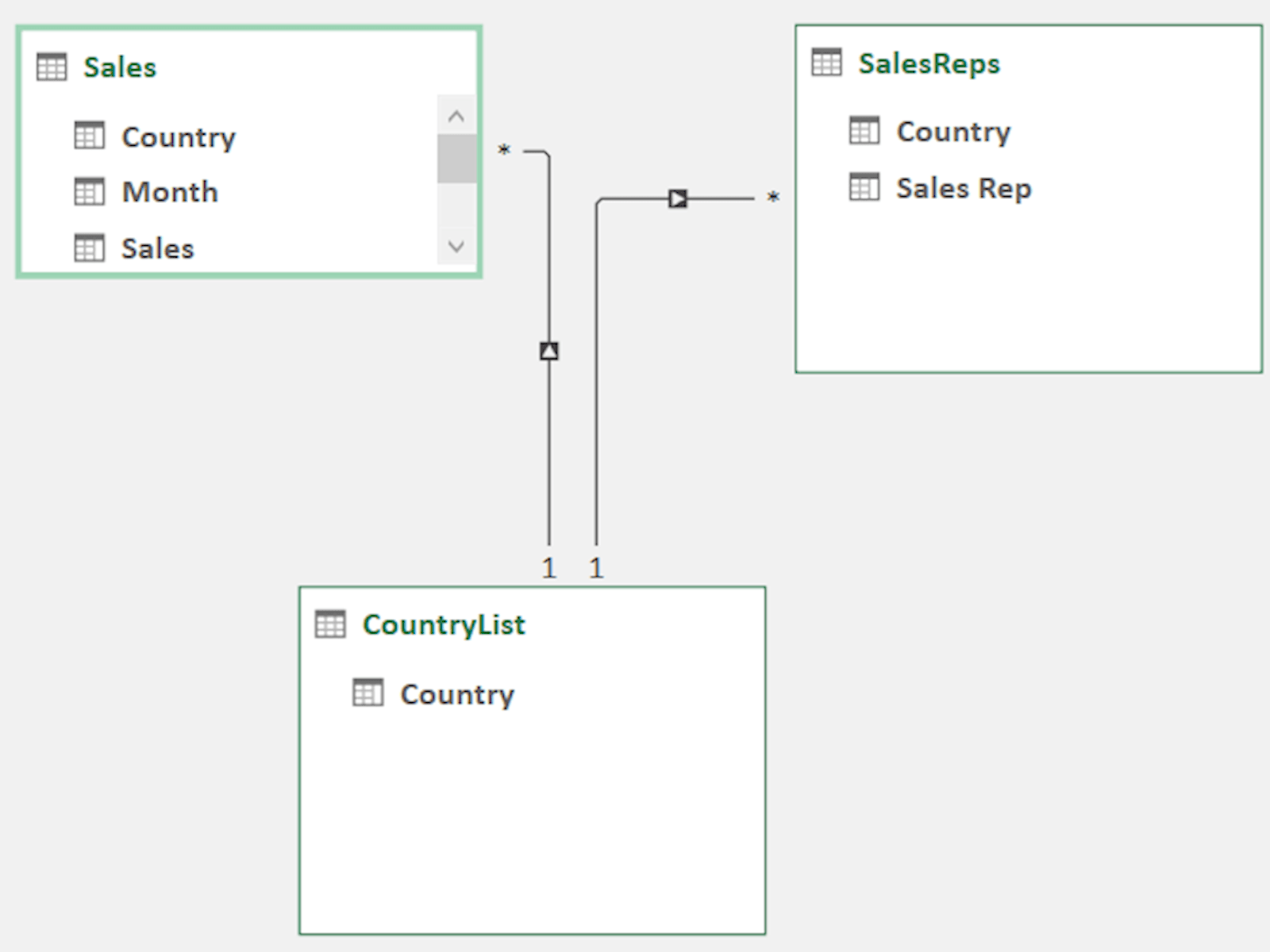
We then import all three tables into Power Pivot, and create connections between them:

We can now create a simple SUMX measure to get our total sales measure:

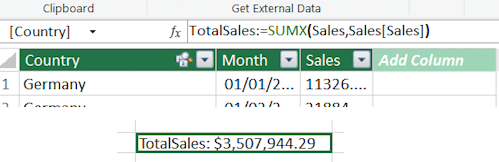
This measure however still won’t work if we try to create a Pivot with the Sales Reps and the Total Sales:

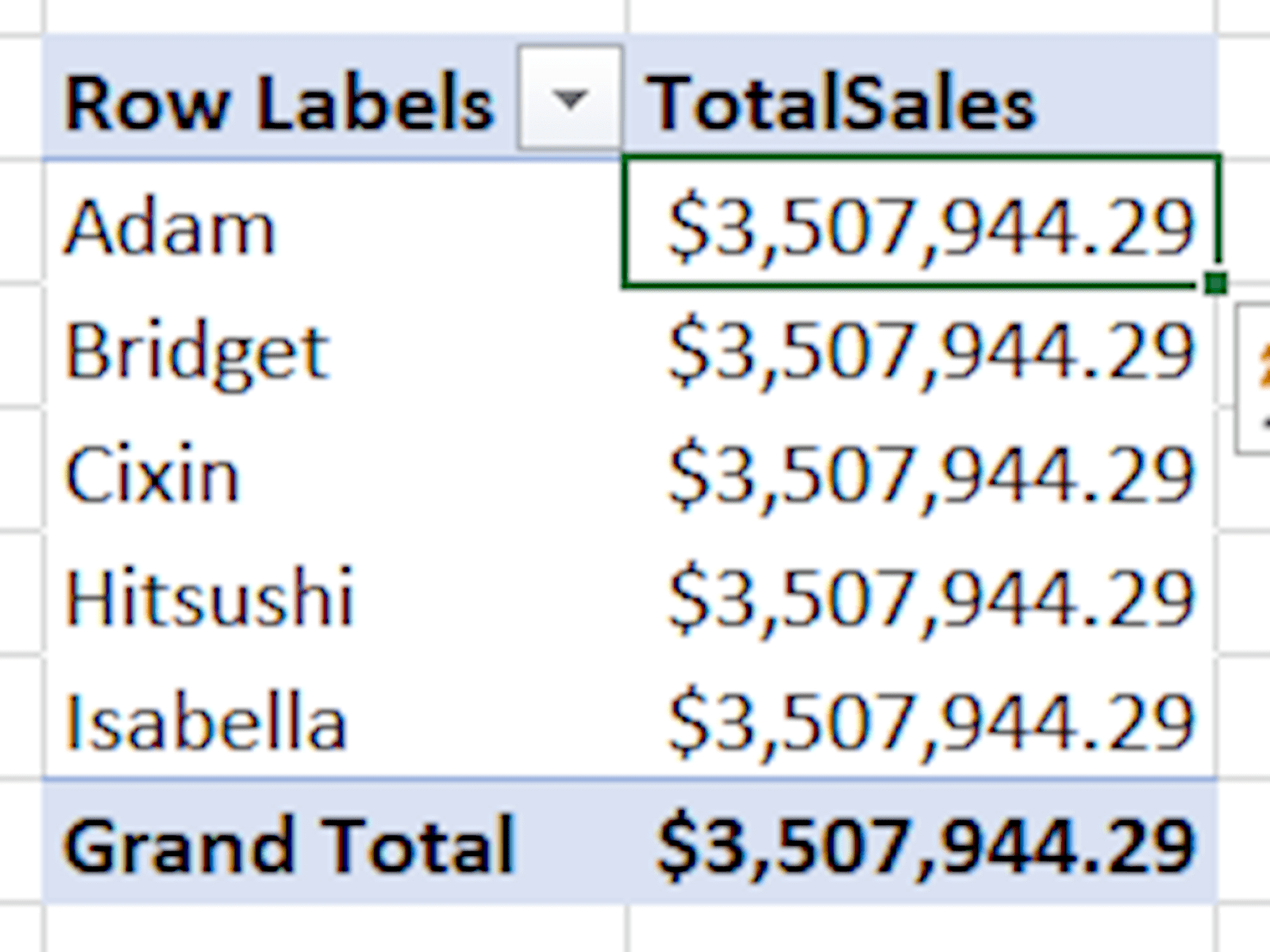
Power Pivot isn’t able to figure out what we want and so the filter context in the Pivot is not applied – all the reps show the full amount.

To do this correctly, we need to use a CALCULATE function to calculate our TotalSales measure over the rows of the SalesReps table. To do this, we use the RELATEDTABLE function, which shows which table we want to use for the connection:

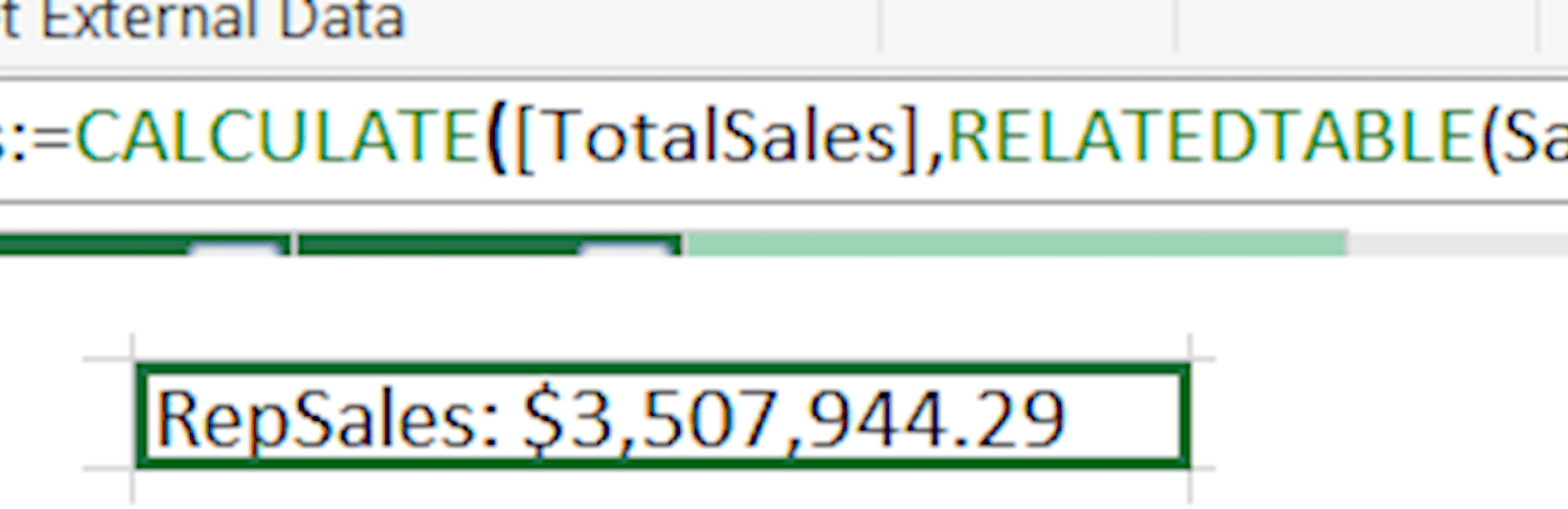
This takes our TotalSales measure, which is tied to the Sales table, and changes up the calculation context to calculate over the SalesReps table instead.  Of course without any context in Power Pivot, the total is the same figure again – but the difference comes when we create a PivotTable on this new measure:

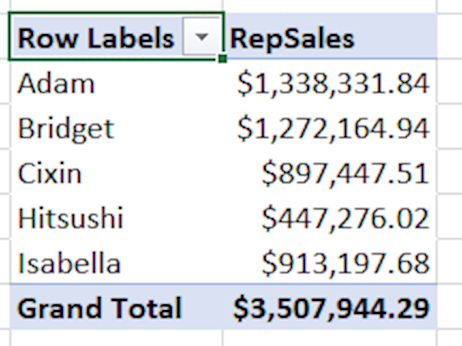
Now we are able to get a total for each sales rep! Note that the grand total doesn’t agree to the total of the individual figures any more, as we are double-counting some figures where a country has more than one active sales rep. But this approach can be used for any kind of situation where there isn’t a straightforward one-to-one or one-to-many relationship between the values in our tables.

Check out the data and the resulting Pivot in the attached workbook.

You may also like

• Previous post - Power Query: Creating transaction references
• TOTW index
• Next time – Revisiting fixing broken links!