Excel Tip of the Week #389 - Power Query: Dropping rows and columns

We have several other posts about Power Query archived in the Tip of the Week Index, so if you want to learn more, check those out.

Dropping rows from your data

Let’s take a look at some sample data:

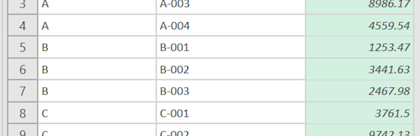
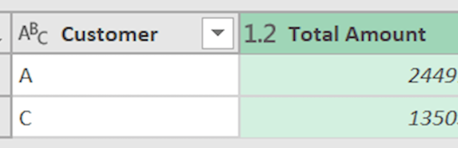
We only want to include customers A and C in our summary data. To do this we simply apply a filter on the Customer column using the dropdown arrow; so long as this filter is still active when we complete our other transformation steps and load the query, then the other customers will be removed. In this case we filter out the other customers and then group by customer:

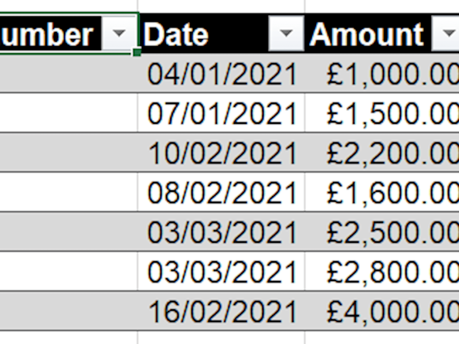
We can also remove rows using automatic operations instead of directly choosing which to include / exclude. Let’s take this table as a second example:

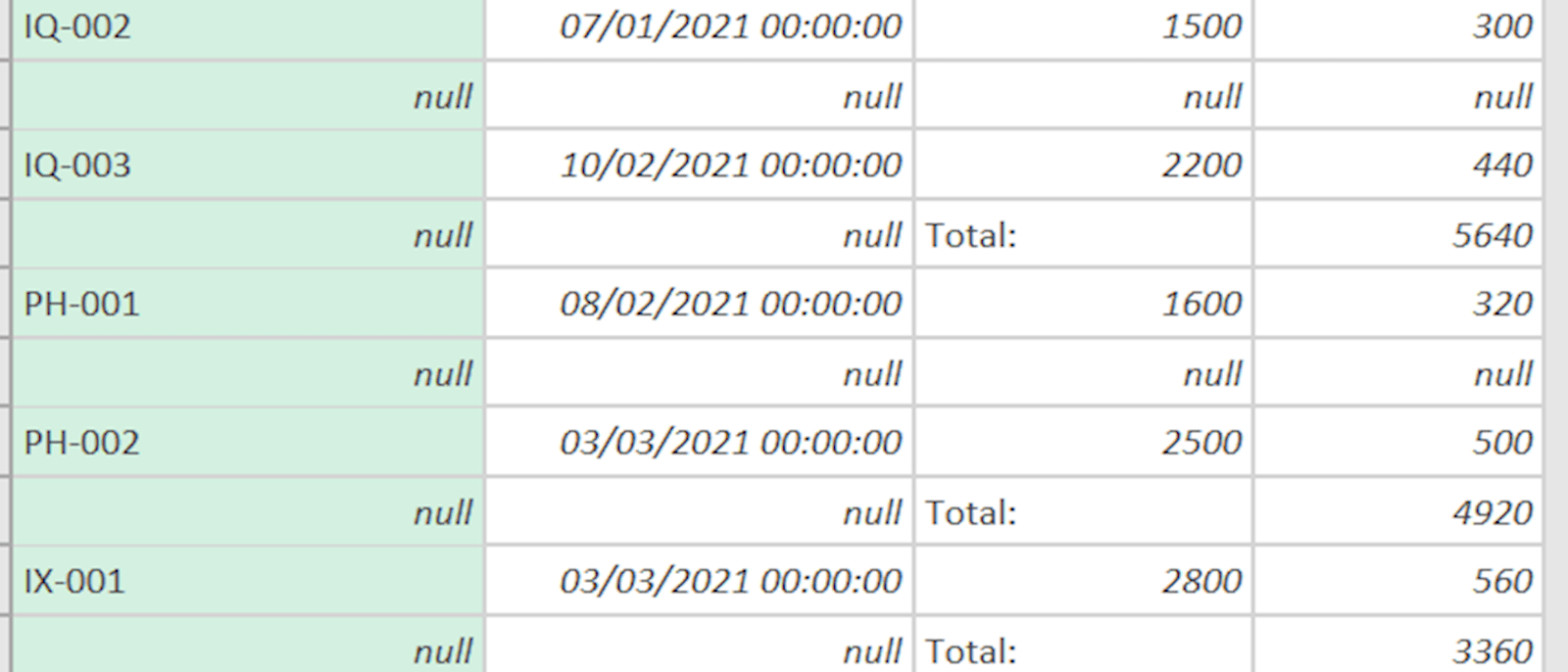
This table has a mixed format – the columns aren’t used consistently, with the customer totals appearing in the VAT column, as well as an unnecessary grand total row at the bottom. We can clean this up using Home => Remove Rows:

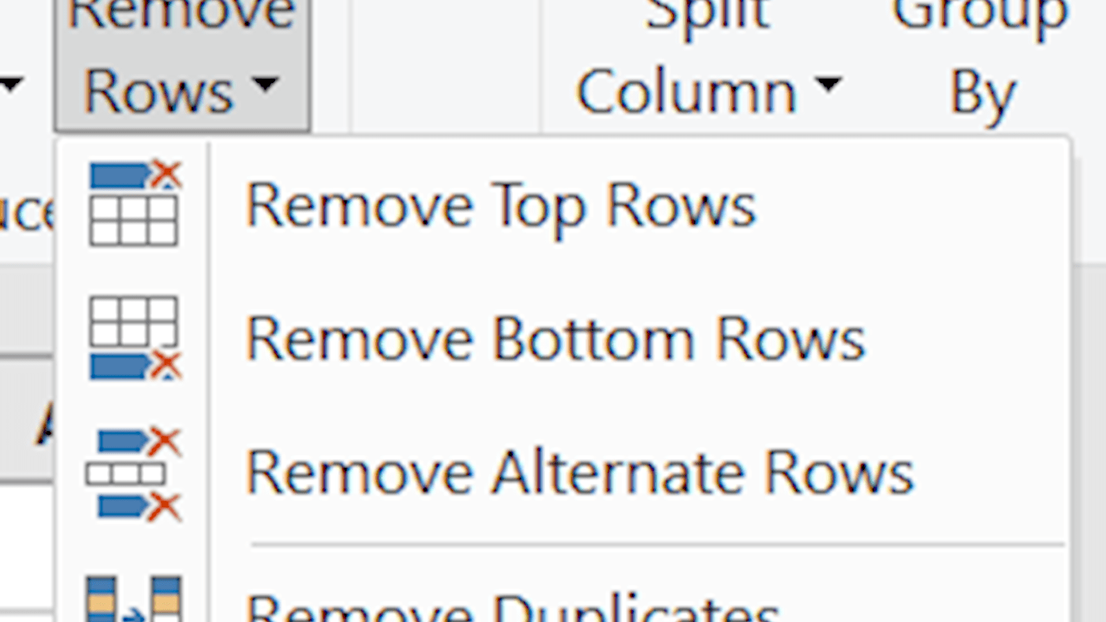
There are several useful options here. For us, we want to remove alternate rows (to clear out the gaps and subtotals, then remove the bottom row (to clear out the grand total row). With that all done, we can then export our sanitised data back into Excel:

As you can see, there are also easy options for removing duplicate rows, rows with errors, blank rows, and so on. These tools can accomplish most common data cleansing tasks.

Removing columns

If instead we want to remove columns, our options are more limited. Let’s look at this example:

If we want to remove columns manually, we can select the ones we want and right click or use the Home menu to either remove those columns, or remove all the other columns. But this lacks the ease and fluidity of a filter, which could act more flexibly, and as-is there is no way to automatically remove e.g. alternating column or the first/last columns as there is with rows. At first things may appear hopeless – but there’s a clever trick!

On the Transform menu, we have the Transpose option. It swaps the rows and columns of the table:

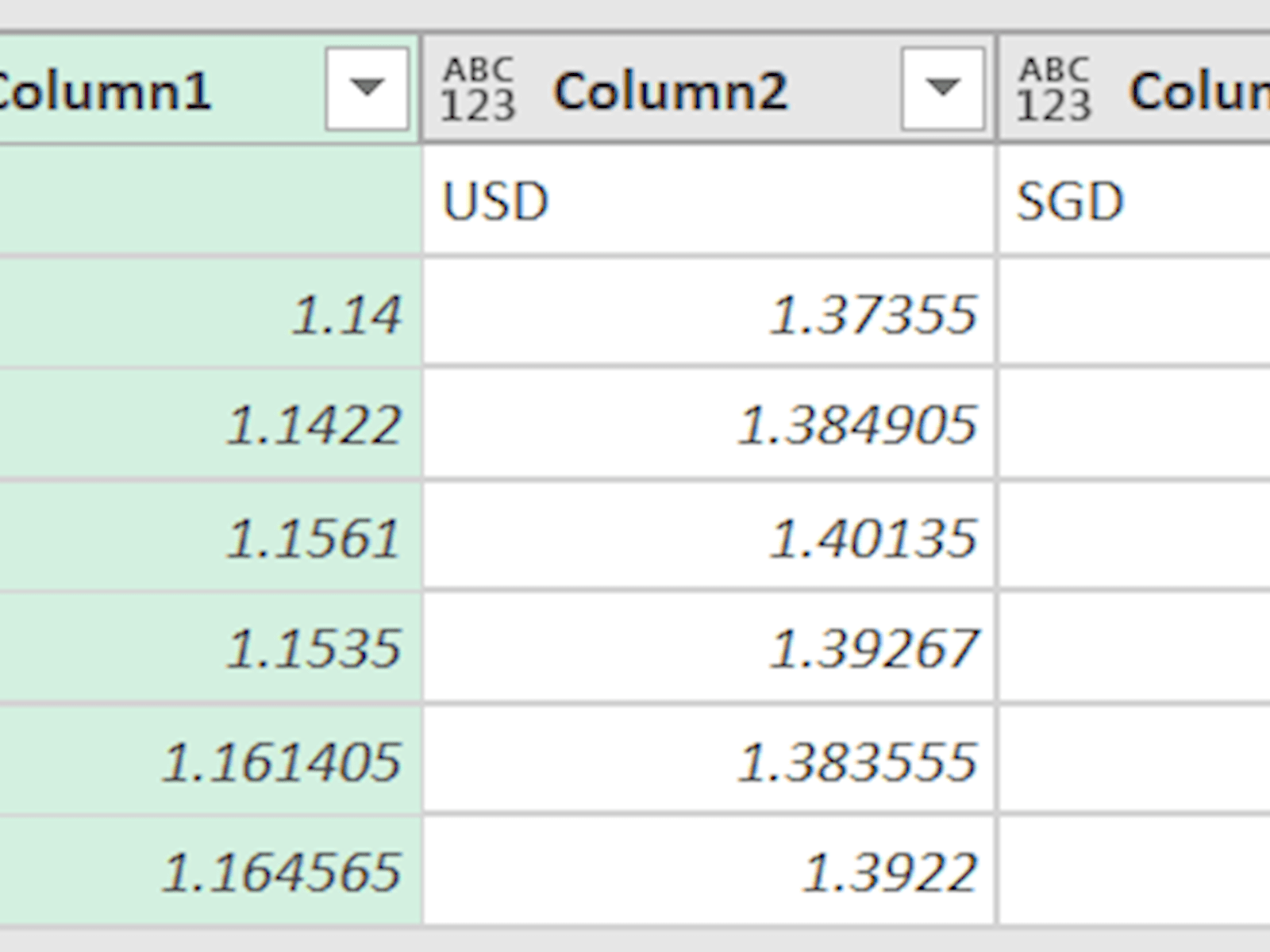
Note that the first column is now the first row, rather than the header row – we could change this using the Transform => Use first row as headers option if we wanted (or indeed do the reverse and move the headers into the first row of data). In this case we will do that to demonstrate how to keep only the most recent exchange rates, for example if this is connected to an automatically growing dataset. We can then re-transpose to restore the original orientation and export:

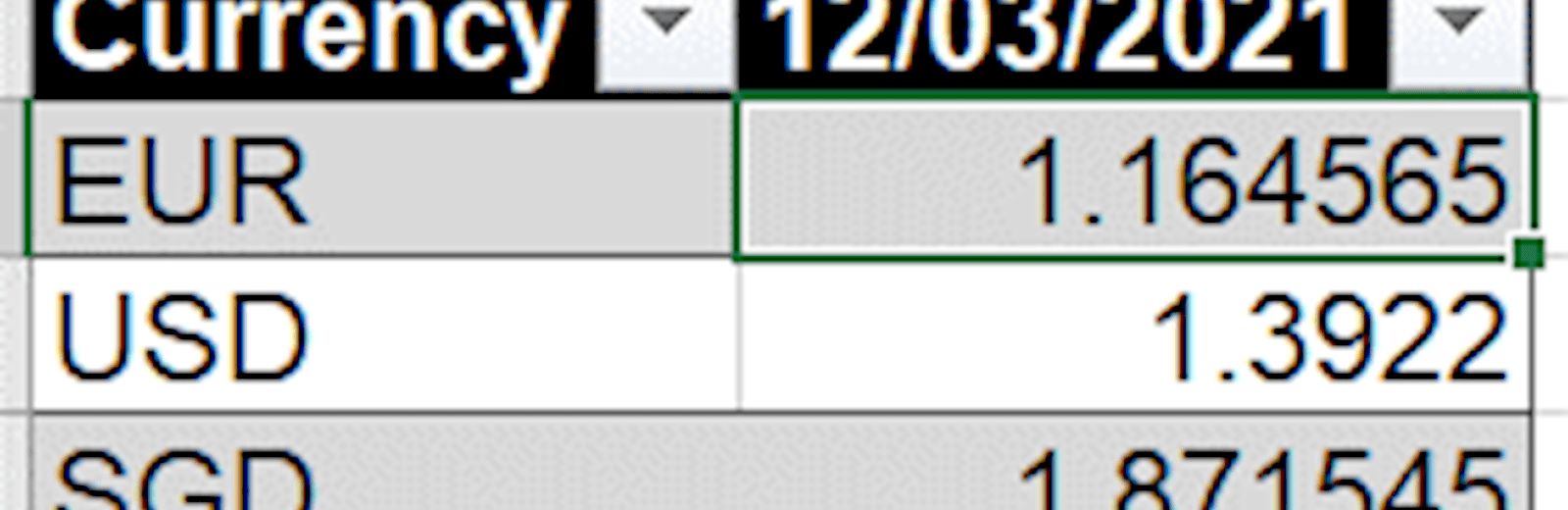
The full process involves demoting and promoting headers multiple times – to follow the full query, check it (and our other examples) out in this accompanying workbook.

• Download the workbook

• Previous Article - 388 - Power Pivot: Filtering measures
• TOTW index
• Next time – Advanced uses of INDEX!