Excel Tip of the Week #406 - Power Pivot: Filtering active contracts

Filtering

We will start by working with this list of contracts and their start/end dates:

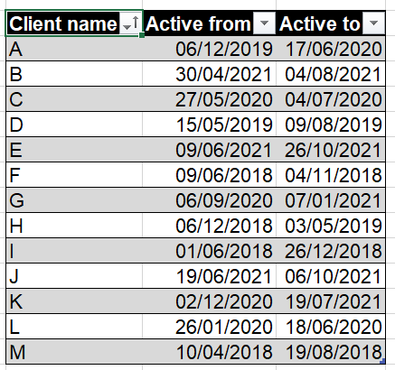
We want to make a simple timeline slicer that will allow us to select any period, and then return a filtered list of which clients’ contracts were active during that period.

To do this, we first insert a Calendar table based on our data – this is done from the Power Pivot window, Design => Date Table => New. This automatically creates a list of every data from the beginning of the earliest year in our data, to the end of the last. This is the list we will use for our Timeline. In this case, we don’t actually need to connect our Calendar to the main data table (which is called Contracts).

Now, we will build a Measure that will return a result for each row telling us whether or not that contract is active during the currently selected period. It looks like this:

InScope:=IF(MIN([Active from])<=MAX('Calendar'[Date]) && MIN([Active to])>=MIN('Calendar'[Date]),1,0)

(note that DAX uses && for the ‘and’ operation, unlike regular Excel which uses the AND function; the equivalent of OR is ||)

This works because the timeline slicer will be based on the Calendar table, and will filter which dates are included to only those in the selected period. We are checking whether the “active from” date falls before the end of the currently selected date range, and the “active to” date falls after the start of that range. It can be a little difficult to intuit that these are the necessary conditions for the contract’s active range to overlap our date period, but if you sketch out the possibilities on a piece of paper it should be clear that this is what we need.

This Measure can now be added to a simple Pivot with a timeline slicer, and we can apply a Value filter that requires the result to be 1:

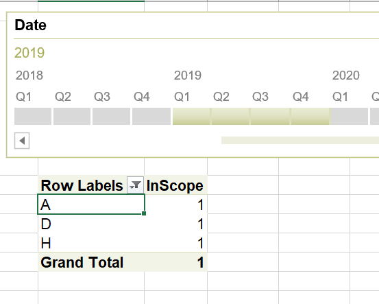
As we can see here, contracts A, D, and H were live during 2019.

Computing

What about if we want to do something else with our data – for example, return a count of active contracts on a specific date, or create a revenue chart?  That’s what we’ll look at next. We’ll use this chart of data:

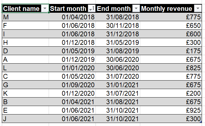
We are aiming to make a monthly summary of how many contracts are active that month, and the total revenue due. That means we will need to make two measures.

Our general approach will be to use the DAX FILTER function to filter the table (this one is called RevenueData), and then calculate what we need to from the results. Let’s start with the number of active contracts:

Active contracts:=COUNTROWS(FILTER(RevenueData, [Start month]<MAX('Calendar'[Date]) && [End month]>MIN('Calendar'[Date])))

The inputs of the FILTER should look familiar from before. This will return a filtered version of the table for each value in our Pivot; we then just use the COUNTROWS function to figure out how big that is.

For our second part, we need to show the monthly revenue. We can use a SUMX to calculate this, but to include the FILTER, this needs to be wrapped in a CALCULATE function – which essentially tells Excel to calculate our SUMX function under the filtering schema we specify. The end result is this Measure:

Total revenue:=CALCULATE(SUMX(RevenueData, [Monthly revenue]), FILTER(RevenueData, [Start month]<Max('Calendar'[Date]) && [End month]>MIN('Calendar'[Date])))

And we can then add both of these into a Pivot:

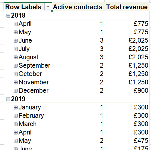
Note that, because we have monthly revenue figures in our original table, and haven’t built anything that checks, while this Measure will work so long as our row labels are months, if we changed it to eg quarters, the Total revenue measure would no longer work – it would instead show the total of the monthly amounts for all the contracts that were active during each quarter.

You can check out both examples in the accompanying file.

• Previous post - DATEDIF redux
• TOTW index
• Next time – Ranking within a group