
We recently held our fourth instalment of our popular series where I answer all of your burning Excel questions live. Despite some Wi-Fi hiccups along the way, we managed to get through a whole bunch of your questions, but there were more we didn’t have time for – so in this article, I will be going through ALL of the questions we received – both those we had time for and those we didn’t!
When entering a formula that refers to another workbook using the Formula Wizard, I have to re-select the other workbook for each input. Is there a way around this?
Not with the Formula Wizard – it’s worth learning to write the function directly into the cell to avoid this problem (and it’s more useful for other things also).
Is there any way of using an IF formula where the logical test relies on text (as opposed to numbers) in certain cells?
Yes, you can make an IF function that cares about text – as part of the logical test, or as an output. The trick is that you have to mark text that’s being entered into a function with speech marks, e.g.:
=IF(A1=”High”, “Avoid”, “Accept”)
I have started to use scenario manager. How am I able to include button for each scenario for users to select the scenario?
Scenario Manager is not a great tool in my opinion, and one of the reasons is how clunky it is to input and switch between scenarios. I would advocate for a simpler formula-based approach. You can read more about different ways to select a scenario in Excel Tip of the Week #319.
Please can you clarify the functional difference between 'hiding' rows vs. using filter selections when it comes to copying values and formats between rows - e.g. when I drag a value or format down multiple rows which are either hidden or filtered?
For almost all purposes, there is no difference between these. But one of the few is one of the ones you highlighted – copying or dragging formulas / values. This will fill cells which are hidden, but not ones which are filtered out. Formats will fill in both filtered out and hidden rows.
Formulas always include all values in ranges regardless of whether some of it is hidden or filtered, with the specific exceptions of the special SUBTOTAL and AGGREGATE functions.
What does the X in XLOOKUP mean?
It doesn’t mean anything in particular – it’s just drawing a comparison with the older VLOOKUP function, which XLOOKUP is intended to replace.
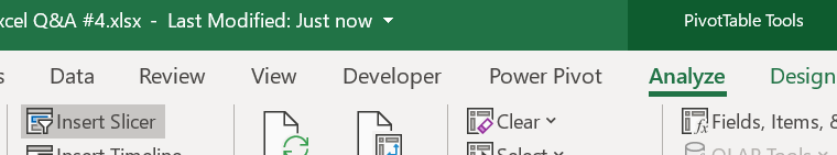
How to you use a slicer on a pivot table?
A slicer is a simple boxout-format filter that you can add to a PivotTable from the Analyze menu for your Pivot:
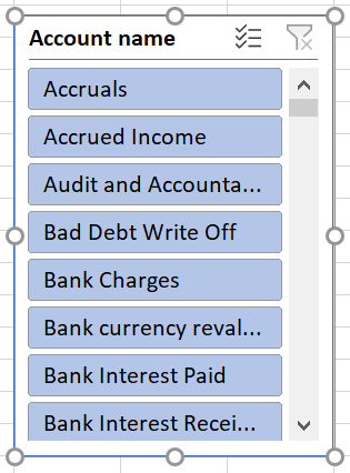
These allow you to quickly and easily filter which rows of the underlying data are included in the pivot.
Using Excel in Office365 it regularly loses the "cut & paste" facility. This can be corrected by closing and reopening the file in question (other open files do not "lose" cut & paste). Is there an explanation of this behaviour?
I am not familiar with this error – it might be worth checking your installation or raising a ticket with Microsoft support.
Which is better, XLOOKUP or INDEX MATCH?
With one caveat, XLOOKUP is definitely superior. The caveat is that XLOOKUP is only in Excel 365 – so if backwards compatibility is a concern, then stick with INDEX MATCH. I did a full comparison of all the lookup functions in TOTW #391.
How do I use Conditional Formatting in situations where I want the format of one cell to be dependent upon conditions existing in a different cell?
You have to write a custom rule using a true/false formula. The trick is to remember to mark the fixed and variable parts of any references with or without $-signs as appropriate so that the rule is correctly applied across your region. For example, here’s a rule that will colour an entire row if the value in column D is over 1,000:
=$D2>1000
In a PivotTable, how do I access the pivot table fields?
If you want to redesign the pivot, you need to see the Field List menu – if this has been closed, select a cell in the pivot and then reenable from the far right of the Analyze ribbon. Or if you want to see the underlying data, just double click any value.
I have a range with column headings with text, say Sales & Costs, and then rows with other headings, say Project 1 & Project 2. I then have a table with the Sales & Costs text in one column and the Project 1 & Project 2 etc. in another column. Is there a way to find the values for the results range? I know I can do this with a pivot table but they are hard to use to report on.
If I am following your question correctly, this can be done with a SUMIFS, by using an INDEX/MATCH with a 0 row input to identify the right column. Here’s the workup:
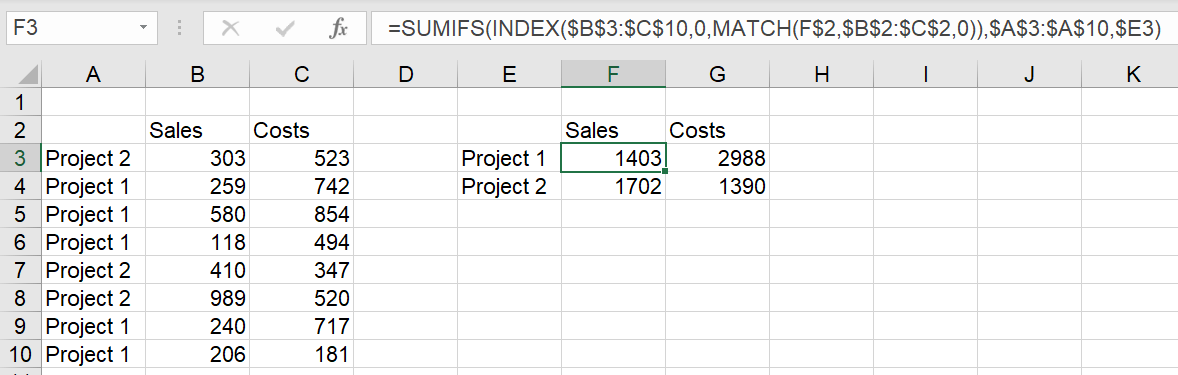
The formula:
=SUMIFS(INDEX($B$3:$C$10,0,MATCH(F$2,$B$2:$C$2,0)),$A$3:$A$10,$E3)
Sometimes when creating a PivotTable, Excel automatically creates time periods (usually quarters) which I find very useful. Sometimes it doesn't.
a) why; and
b) if it doesn't summarise by quarter for me, how can I do that (other than changing the base table)?
The automatic grouping is a bit hinky – there’s no clear explanation for why it does and doesn’t happen. However you can add / remove / change it by right clicking on one of the field headers and using Group/Ungroup.
What would you suggest are the key features/actions in Excel that a trainee accountant should be able to use?
Here I would refer to our Spreadsheet Competency Framework. I would expect most trainees to aim for the General User level, with Creator level as an aspirational goal.
Can you run through Power Query, and how it can be best used for financial accountants?
Power Query is an extract-transform-load (ETL) program designed to help you automate repetitive data transformation tasks. It comes free with Excel and can be used to bring in data from a table, file, or folder, perform a pre-recorded series of steps to transform it, and then output as a table or pivot in Excel. It’s great for data cleaning, combining data from multiple files, and other common data manipulation tasks.
We have several webinars in the archive that might help – I’d suggest this introduction to PQ from last year as a good place to start. We will be running this one on everyday PQ tasks in June.
Is there a charge for this Power Query webinar?
Yes, these webinars are part of the Excel Community member offering.
How do you easily select a large section of data?
If the data has a blank column and row after it, Ctrl A can do this. Or you can manually zip through data and select it by using Ctrl Shift + arrow keys.
What's the easiest way to remove duplicate values in a column so that only one of each value remains?
You can do this with Data > Remove Duplicates, or in Excel 365 with the new UNIQUE function.
Is there a shortcut to select the whole of the row you are in? I work with wide datasets and if I am on one side of the sheet can be hard to see which cells across the sheet relate to it.
Shift Space does this, and Ctrl Space selects the current column. You might also want to investigate Home > Format as Table, which can make tables with alternating banded rows that are much easier to read across.
How can I create an IF for when a date falls in between 2 dates?
You need to test the date cell against each condition independently, and combine the results with an AND function. An example might be:
=IF(AND(date cell >= start date, date cell <= end date), output 1, output 2)
Note that the start and end dates should be entered either into their own cells, or with the DATE function.
PivotTable date data is sometimes text not date. Is there a quick way to get this all in date format so it can be summarised in the pivot table?
This most commonly happens when some cells have been marked as Text format. You can change the format, but Excel won’t notice until you click into the cell to fix it. You can automate this “clicking in” process by doing a find & replace on something like “replace / with /”, which won’t actually change anything but will kick Excel into noticing that you have dates.
Is power query available only in Office 365?
No, it has been around for a long time. The Mac version is still not fully-featured, unfortunately.
If I have two different tables, where column A contains the same set of data in both (but each may only contain part of the data in the other column A) and I need to line up the data in the B columns against the data in column A - one set in column B and the other in a new column C, how would I go about this please?
This is a textbook case of using the Power Query Merge function – load both tables into PQ first, and then use the Merge operation:
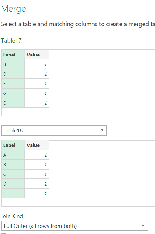
Note the join kind is “Full Outer” – this will ensure your merged version has all the rows from both tables.
Regarding date groupings in pivots, how can I arrange the months to run in FY rather than calendar years? So the year would run April to March.
This is unfortunately a little more complex to do than I would like.
We need to add two formula columns to the underlying data to compute the fiscal year and fiscal month. Here’s a look at that:
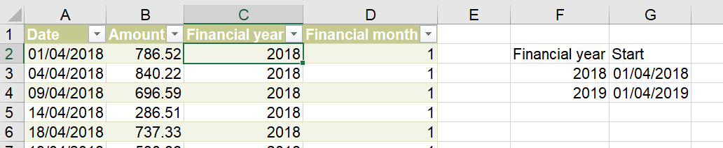
The formulas are:
=INDEX($F$3:$F$4,MATCH(A2,$G$3:$G$4,1))
=MOD(MONTH(A2)-4,12)+1
The first one is a lookup that find the appropriate financial year based on the table on the right; the second mathematically moves the month number back by 3.
This lets us create a pivot with the fiscal year ordering:
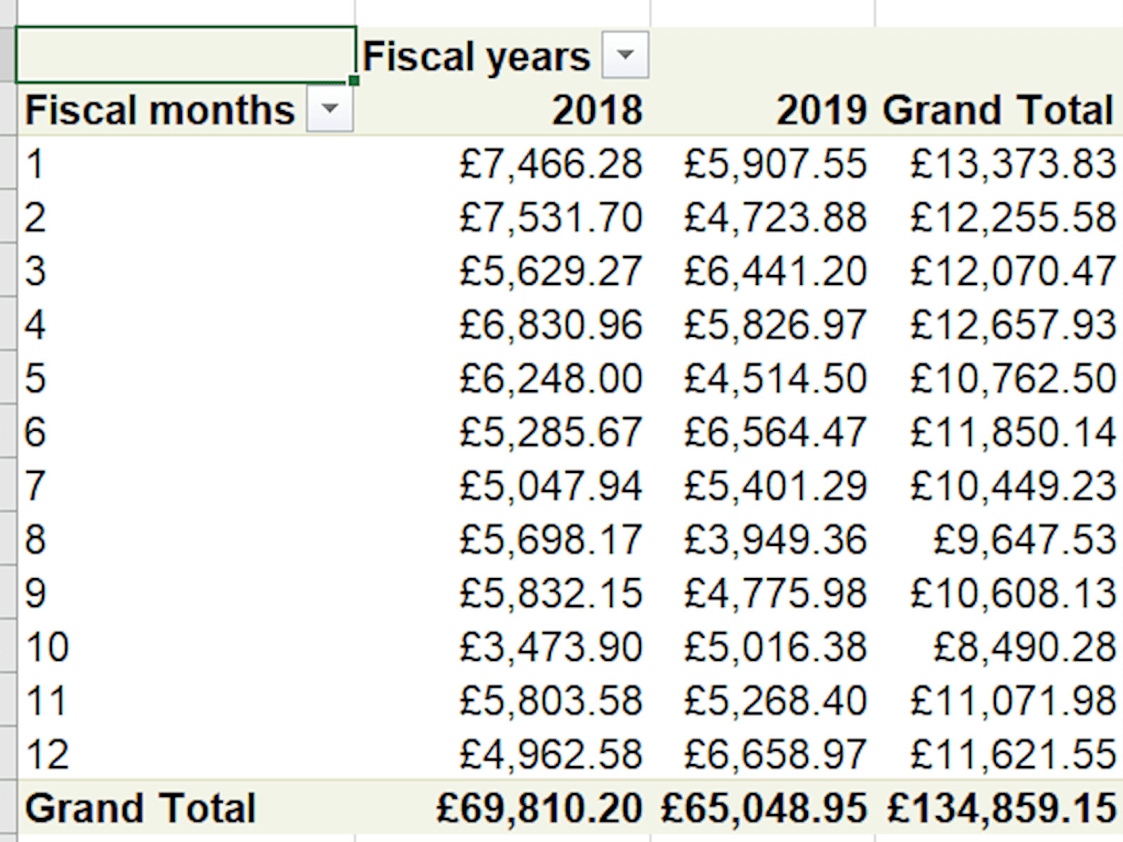
It’s a bit of a pain to set up, but once created should automatically work from there on.
Are there any sessions planned for Power Pivot? I really struggle with this especially how to link tables.
We have one in the archive on how to get started:
Excel community
This article is brought to you by the Excel Community where you can find additional extended articles and webinar recordings on a variety of Excel related topics. In addition to live training events, Excel Community members have access to a full suite of online training modules from Excel with Business.

Archive and Knowledge Base
This archive of Excel Community content from the ION platform will allow you to read the content of the articles but the functionality on the pages is limited. The ION search box, tags and navigation buttons on the archived pages will not work. Pages will load more slowly than a live website. You may be able to follow links to other articles but if this does not work, please return to the archive search. You can also search our Knowledge Base for access to all articles, new and archived, organised by topic.