Key takeaways
- Search and return in Excel XLOOKUP: The Excel XLOOKUP function builds on the previous VLOOKUP and INDEX and MATCH functions by combining the search and return steps.
- XLOOKUP match_mode: While XLOOKUP uses an exact match by default when searching Excel spreadsheets, match_mode controls whether Excel uses an exact, approximate or wildcard match.
- Multiple matches and XLOOKUP: XLOOKUP can return more than a single cell if there is more than one match. The result can spill into neighbouring cells as an array output.
Looking up information is one of the most common jobs in Excel. You might, for example, have a customer code and need to find a customer name, invoice number and a product. Or you might have a score and need the corresponding grade.
For years, Excel users relied on VLOOKUP or the INDEX and MATCH combination. XLOOKUP brings the search and return steps together in one modern function that offers some serious flexibility.
The anatomy of XLOOKUP
=XLOOKUP(lookup_value, lookup_array, return_array, [if_not_found], [match_mode], [search_mode])
- lookup_value is the item you want Excel to find.
- lookup_array is the row or column Excel searches.
- return_array is the row or column containing the result you want back.
- if_not_found is an optional message or value to return when no match exists.
- match_mode controls whether Excel uses an exact, approximate or wildcard match.
- search_mode controls the direction or method of the search.
Using required arguments (1-3), and optional argument (4), a simple lookup might be:
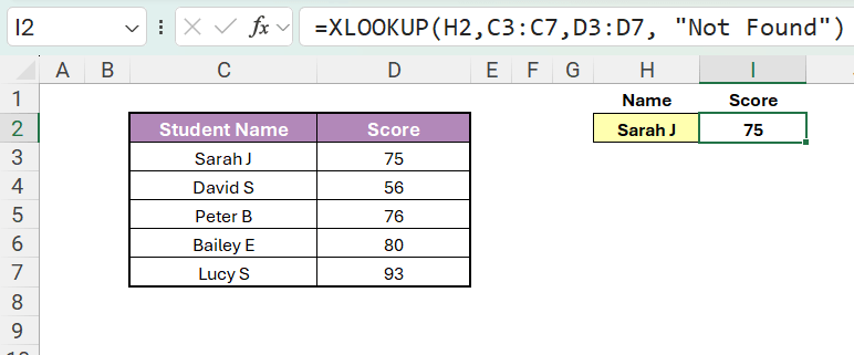
In the example above, Excel searches for the value in H2 (“Sarah J”) within C3:C7 and returns the corresponding value from D3:D7. If no match is found, it displays “Not found”. Here, Sarah J scored 75, so the result 75 is returned.
Using optional argument (5) to determine match mode
XLOOKUP uses an exact match by default (unlike VLOOKUP or HLOOKUP), but the optional match_mode argument gives you four choices:
| Match mode | What it does |
| 0 | Exact match. This is the default. |
| -1 | Exact match, or the next smaller item if there is no exact match. |
| 1 | Exact match, or the next larger item if there is no exact match. |
| 2 | Wildcard match using *, ? and ~. |
Approximate matching
Approximate matches are useful for banded tables such as grades, tax rates or discounts. Suppose a grading table contains these lower boundaries:
| Score | Grade |
| 0 | Fail |
| 60 | D |
| 70 | C |
| 80 | B |
| 90 | A |
To return the grade for a score in cell F2 in the example below, we’d use:
=XLOOKUP(F2,C2:C6,D2:D6,,-1)
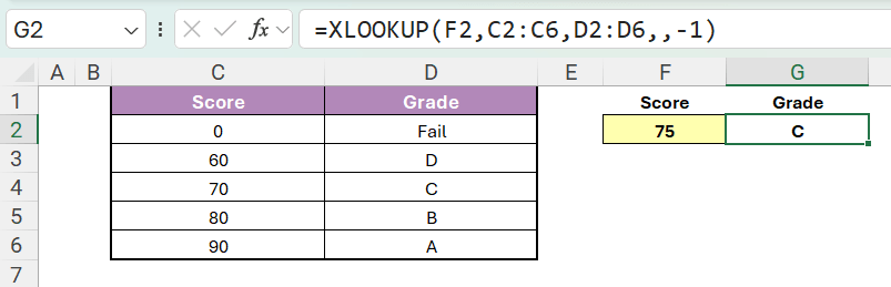
Let’s say F2 contains 75, and there is no exact value of 75 in the score column. Match mode -1 tells XLOOKUP to use the next smaller item, which is 70, so the formula returns C. Keeping the thresholds in a table makes the logic easier to review and maintain than a deeply nested IF formula.
Wildcard matching: searching with only part of a value
Wildcard matching is useful when you know only part of the text you are looking for. Set match_mode to 2, then use one of Excel’s wildcard characters in the lookup value:
| Wildcard | Meaning | Example |
| * | Any number of characters | "South*" |
| ? | Exactly one character | "INV-1000?" |
| ~ | Treat the next * or ? as a literal character | "Product~*" |
For example, as shown below, using a football dataset where team names sit in C2:C6 and goals scored sit in D2:D6:
=XLOOKUP(F2,C2:C6,D2:D6,”Not Found”,2)
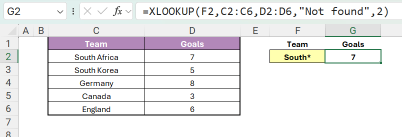
The asterisk (*) you see after “South” in the yellow input cell (F2) means “any number of characters”. Excel therefore looks for the first team name beginning with “South” and returns that team’s goals scored. As South Africa appears before South Korea in the lookup range, South Africa is the result because XLOOKUP returns the first match it encounters by default.
A question mark matches exactly one character. For example:
=XLOOKUP(F2,C2:C6,D2:D6, “Not Found”,2)
This could match INV-10000 through INV-10009, but not INV-100000, because the question mark stands for one character only. If you genuinely need to search for an asterisk or question mark stored in the data, place a tilde before it, such as Product~*.
Using optional argument (6) search mode: controlling where Excel starts
The optional search_mode argument controls the direction or method of XLOOKUP’s search:
| Search mode | What it does |
| 1 | Search first to last. This is the default. |
| -1 | Search last to first. |
| 2 | Binary search on data sorted in ascending order. |
| -2 | Binary search on data sorted in descending order. |
The most useful alternative to the default is -1, which searches from the end of the lookup array, back towards the start.
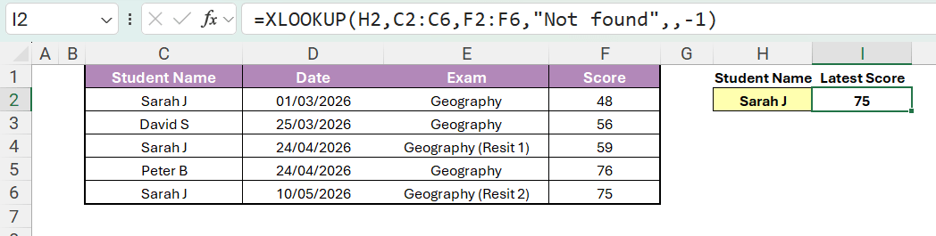
Imagine a student appears several times in a list of exam scores within a table and you want the most recent entry, with the newest scores stored at the bottom of the list:
=XLOOKUP(H2,C2:C6,F2:F6, “Not found”,,-1
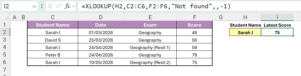
The -1 in the final argument tells Excel to start at the bottom and work upwards, so the last matching record is returned without having to reverse the dataset.
It is unlikely you will need to turn to binary search modes in your regular work, so we’ll leave those out of this article on that basis.
Returning arrays if there are multiple matches
XLOOKUP does not have to return a single cell. If the return_array covers more than one column or row, the result can spill into neighbouring cells as an array output.
=XLOOKUP(H2,C2:C6,D2:F6, “Not Found”)
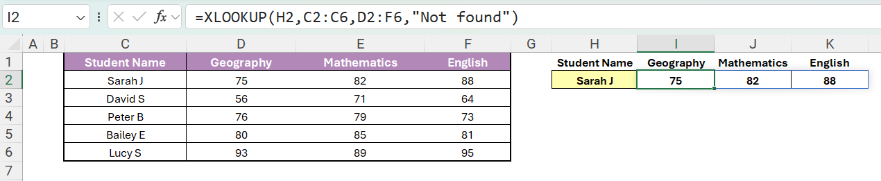
In the example above, Excel searches for the value in H2 within C2:C6, and returns matching values from columns D to F (75;82;88).
Final thoughts
XLOOKUP is one of the most versatile functions in Excel and is a “must” in every Excel user’s toolkit. INDEX / MATCH (or XMATCH) is still a firm favourite for many people, and that’s absolutely fine, but in most situations XLOOKUP does just as much, or more, within a single function.
Excel tips and tricks
ICAEW's Excel Community shares regular Tips & Tricks on how to get the best out of this key accountancy tool. See all their posts by topic, and by level in the Spreadsheet Competency Framework.

You may also be interested in
ICAEW Community

Excel
Do you use Excel in your organisation? Are you using it to its maximum potential? Develop your skills and minimise spreadsheet risk with our Excel resources. Join the Excel Community
ICAEW Certificate

Analytics in Power BI
Gain essential data analytics skills and advanced reporting techniques to stay ahead of industry demands with this practical qualification from ICAEW.
Find out moreICAEW support

Training and events
Browse upcoming and on-demand ICAEW events and webinars focused on making the most of the latest technologies.
Events and webinars CPD courses and more