Excel Tips and Tricks #448 – A Distinct Count Conundrum

Setting the Scene

Imagine this – you have 4 clients, and you want to produce a list of which accounting systems they use (Sage, Quickbooks, Xero, Netsuite and so on). A quirk of this piece of MI is that it is a many-to-many relationship; multiple clients might all use the same accounting system, but equally one client can, on occasions, use multiple different systems:

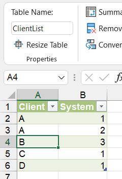
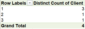
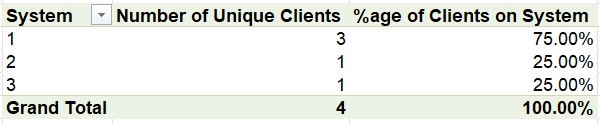
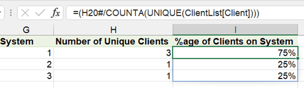
If I wanted to summarise this, I could easily show that 3 clients use system 1, 1 client uses system 2 and 1 client uses system 3. But what if I want to show the percentage of clients on system 1? Because client A uses two different systems, the calculations become more complicated. System 1 appears 60% of the time in our table, but is actually in use at 75% of the clients. Systems 2 and 3 only appear 20% of the time in our table, but each is in use at 25% of our clients.

Solving this for 4 clients might be easy enough, but if you are dealing with MI relating to dozens, hundreds or even thousands of clients across your audit firm, and many different accounting systems, this can become a big challenge. There are however a couple of different solutions to this conundrum…

Pivot Tables 1 – Add to Data Model

First things first – I’ve taken my data and turned it into a table (select the data and press Ctrl+T), calling it “ClientList”:

There is a somewhat hidden feature of pivot tables that allow you to calculate a distinct count. However, in order to do this, you have to select the “Add this data to the Data Model” option when creating the pivot table:

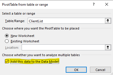
It’s not entirely clear why the distinct count option only becomes available when this is ticked, such are the quirks of Excel. But, with your dataset in the data model, getting the percentage of clients is just a few easy clicks away:

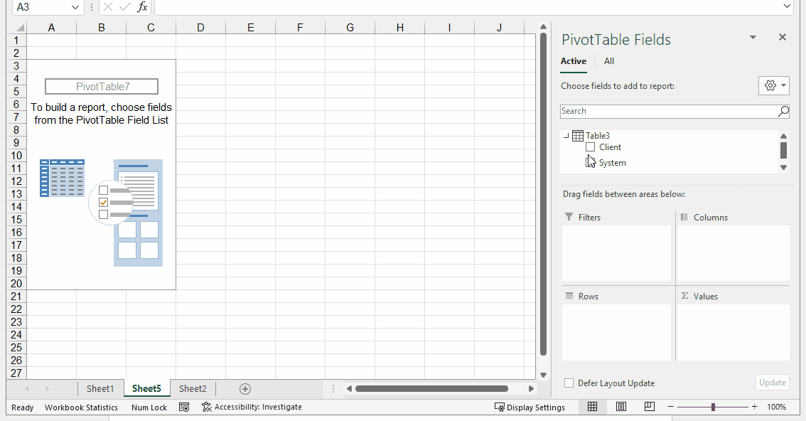
• Add “System” to rows
• Add “Client” to values
• Go to the Value Field Settings
• Select “Summarize value field by” Distinct Count
• Select “Show Values As” % of Grand Total

Now, there are some things to watch out for – not least the obvious issue here that the “Grand Total” doesn’t equal the sum of the percentages (which would be 125%). However, this total reflects the total number of clients, which is 4, and so while it looks odd, it is showing the “right” number.

A little tidying up and you can fairly quickly get to a finished table:

There is of course the perennial annoyance of pivot tables not refreshing automatically – though another hidden tick box in PivotTable Options, below, might help at least a little with this:

Pivot tables can be annoying in many other ways, so if you’re not a fan, why not do it another way…

Dynamic Arrays

With our newfound love of dynamic arrays (see last week’s introductory webinar Hooray for Arrays), there is of course a solution here which recreates the trusty pivot table.

To generate the summary System column, we can just use the UNIQUE array function:

Generating the number of unique clients on each system can then just use the COUNTIF function as a dynamic array:

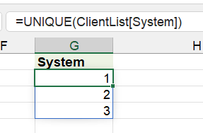
Note here that, Excel has automatically populated the formula just by my selection of the relevant cells; I did not type “G20#” but I selected the range G20 to G22 and that’s what Excel gave me. Clever, eh?

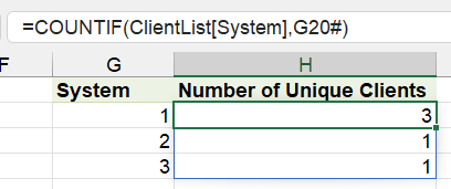
The last step, to get the percentage of clients on each system, simply involves taking the number of unique clients for each system and dividing this by a count of all the unique clients in the source table; COUNTA kindly accepts an array input, so we can use that in combination with UNIQUE again, but this time on the “Client” column:

OK, you have to set the column format as percentage (select the cells and press Ctrl+Shift+%). And that’s the annoyance of dynamic arrays, that you have to manually set the formatting (unless you can do some wizardry with conditional formatting of course – that’s for another day). But on the flip side, if you add more clients and systems to your main table, the dynamic array will automatically grow and update:

Conclusion

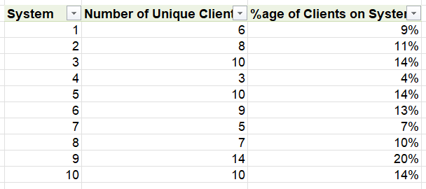
This is of course a very specific scenario, but not necessarily an unusual one. While there are pros and cons to either solution (and probably many more solutions to boot), this tip can hopefully help in any situation where you require distinct counts and percentages of total populations, where your data has a many-to-many relationship. Happy Excel-ing!