Excel Tip of the Week #391 - Comparing the lookup functions

We’ll be covering the gist of them, but if you want a bit of background reading on the functions covered here, check them out in our archive as follows:

• VLOOKUP – TOTW #168
• INDEX MATCH – TOTW #201
• XLOOKUP – TOTW #337

What's in a lookup? 

Let’s review the basics with a look at what a lookup is and what it’s for.

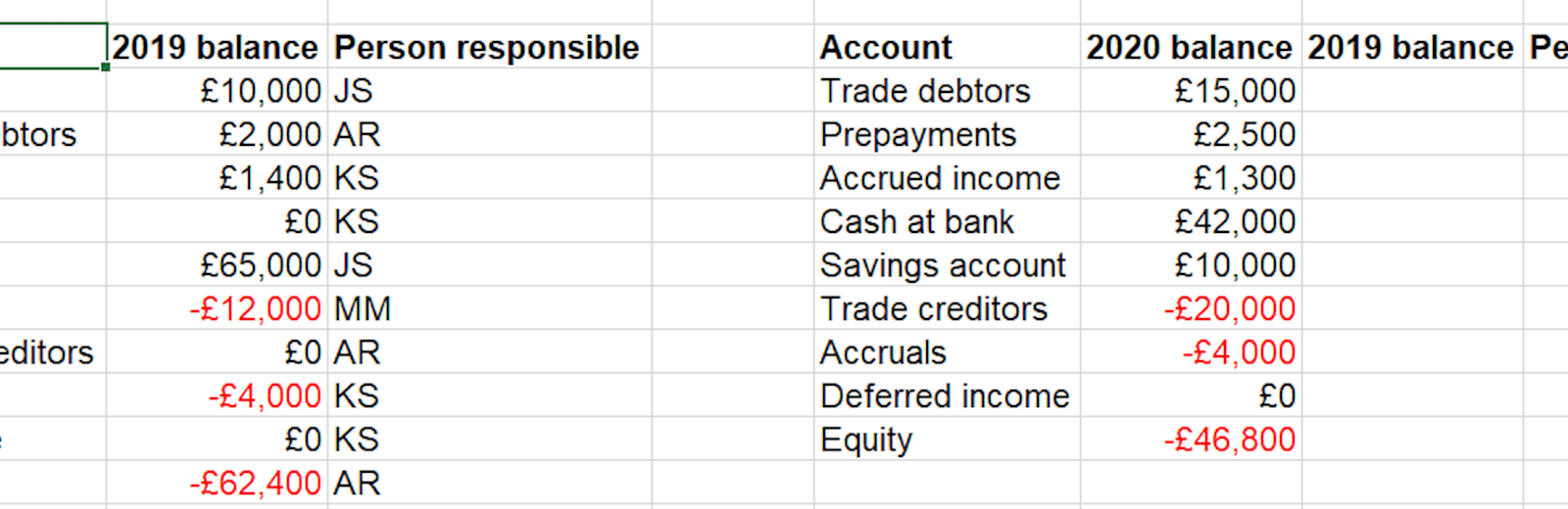
Here we have a master data source (on the left), and then on the right we have a new location where we want to import information from that data source. The two are connected via some kind of unique label or identifier. The data we want to pull could be numeric (such as the 2019 balances), or it could be non-numeric (such as the initials of the staff member responsible for that area). All lookup functions share these qualities:

1. They work with either numbers or text
2. They rely on a unique identifier, and will not work if identifiers are repeated
3. If searching for an identifier that is not present, they will either return an error or another nearby value depending on the circumstances and how the functions are written

As well as the three above functions, we’ll also be examining LOOKUP. This is an old Lotus 1-2-3 function that’s still usable in Excel for backwards compatibility reasons, but as we will see it is generally not a great choice.

Handling of unsorted data

If your data in unsorted, how will the different functions handle it?

LOOKUP – will not work

VLOOKUP – will work only if the FALSE option is specified

INDEX MATCH – will work only if the 0 option is specified

XLOOKUP – works by default

This is the single big strike against LOOKUP – it only works if the unique identifiers are sorted into order; otherwise it will return incorrect results.  VLOOKUP and INDEX MATCH can both handle this situation, but annoyingly their default behaviour is to assume the data is sorted and find an approximate match.  XLOOKUP automatically looks everywhere for your result.

Ease of writing

How easy are these functions to input?

LOOKUP – Easy; can directly point at label and value columns
VLOOKUP – Hard; have to select entire data range and count which output column is desired

INDEX MATCH – Medium; have to embed one function within another

XLOOKUP – Easy; can directly point at label and value columns

VLOOKUP suffers the most here, because not only does the entire data range have to be selected, you also have to manually count across to identify which column you want the function to return.  INDEX MATCH is also a bit trickier as it requires nesting a MATCH function inside an INDEX function.

Handling of labels not on the left

If your data is not laid out with the labels on the left, how does that affect things?

LOOKUP – Works normally

VLOOKUP – Does not work

INDEX MATCH – Works normally

XLOOKUP – Works normally

Because of the “table array” input in VLOOKUP, it can only handle data where the labels are the leftmost column.

Handling of insertion / deletion of columns

LOOKUP – Unaffected

VLOOKUP – Breaks

INDEX MATCH – Unaffected

XLOOKUP – Unaffected

In another strike against VLOOKUP, because the output column is manually identified through the “column index no”, if columns are inserted or deleted from the data range later on, the VLOOKUP will break.

Handling of horizontal lookups

LOOKUP – Works

VLOOKUP – Has to be replaced with HLOOKUP

INDEX MATCH – Works

XLOOKUP – Works

All four of these families can handle a horizontal lookup – that is, searching along a row for an identifier – although the vertical VLOOKUP has to be supplanted with its sister function HLOOKUP.

Returning multiple values

If we want to use one identifier to return several values, how easy is it to do that?

LOOKUP – Medium – have to set up $-references carefully

VLOOKUP – Hard – have to increment column index number manually or with a COLUMN function

INDEX MATCH – Medium – have to set up $-references carefully

XLOOKUP – Easy – Can return a spilled range of values

VLOOKUP struggles once more, as the need for a direct column index number means that returning more than one value will involve some added complication.  INDEX MATCH and LOOKUP can both be copied rightwards with only minor alteration, and XLOOKUP, being a dynamic array function, can directly return multiple values by selecting a wider array for the “return array” input.

Searching for multiple input values

LOOKUP – Simple copying

VLOOKUP – Simple copying

INDEX MATCH – Simple copying

XLOOKUP – One function

Similarly, all the older functions can be used to look for multiple different identifiers by means of a simple copy and paste (with appropriate $-references); however XLOOKUP can also look up an array of inputs with a simple formula.  Note that unfortunately you can’t combine this with the above.

Error handling

If no match is found, how is this handled?

LOOKUP – Finds another value based on proximity or returns #N/A!

VLOOKUP – Returns #N/A!

INDEX MATCH – Returns #N/A!

XLOOKUP – Can be customised to show any desired value

Generally the older lookup functions will return a “not applicable” error if they cannot find an exact match; the IFERROR function is often used to replace this with a custom error message or other function. XLOOKUP has a “value if not found” input built directly into the function.

Availability

Which versions of Excel support which functions?      

LOOKUP – Lotus 1-2-3 and all Excel versions
VLOOKUP – All Excel versions
INDEX MATCH – All Excel versions

XLOOKUP – Excel 365 only                

While easily the best function for lookups, XLOOKUP is only available for Microsoft 365 or Excel Online users. Those with Excel 2019 or earlier will not have access.

In conclusion

If I had to summarise all the above into a single recommendation, it would be this: if you and your collaborators all have access to it, use XLOOKUP; otherwise, use INDEX MATCH. And always think about what you’re trying to do is a lookup at all, and if not, consider using something like SUMIFS or a PivotTable instead.

You can check out demonstrations of all four alternatives in the accompanying file.

You may also like

• Previous post - Advanced uses of INDEX
• TOTW index 
• Next time – 392 - Text to Columns redux