Excel Tip of the Week #429 - Revisiting cross-sheet formulas

The basics

A reference to another worksheet looks like a reference within the same sheet, with a little extra to specify which sheet is being referenced. There are two variations that you will see:

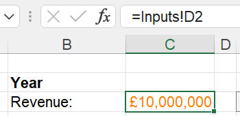
For a sheet with a single word name, the name of the sheet is simply listed, followed by an exclamation mark and then the cell(s) being referenced.

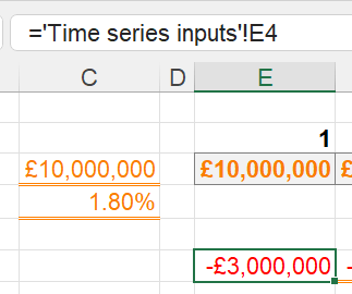
For sheets with multiple words in their names, the sheet name is wrapped in a set of single quotes. The exclamation mark part remains the same.

Note that cross-workbook references build on this same model – see this reference to another workbook which is currently open:

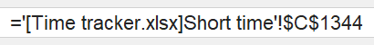
And the same reference when the other workbook is closed:

In either case the filename is included in square brackets before the sheet name; if the other file is closed then the full file directory is also included.

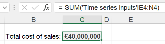
The same syntax also works for references to ranges of cells on other worksheets; if you don’t have Office 365 or 2022 then you will need to include some kind of summary function in one of these:

3D references

You can expand further upon this idea by creating what is called a 3D reference. Just like a range can refer to a block of cells that lies between two addresses (like E4:N4 above), a 3D reference can refer to the same block of cells across a selection of adjacent worksheets. There are some wrinkles that make them a little tricky to work with, but for starters let’s look at how they work. Starting with adding up a single cell from each sheet:

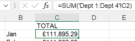
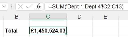
Essentially you just append the first and last sheet names using a colon, the same way you would for a range of cells, inside the single quotes. The same approach can be used for ranges of multiple cells across multiple sheets:

Now, as mentioned, this isn’t a perfect approach. Of course it relies on all your individual sheets having identical layouts – which isn’t easy to check. Adding a row to one of the sub-sheets would lead to a material issue but be easily missed.

Secondly, because the first and last sheets are directly named in the formula, rearranging the sheets will change the results. If another sheet is added in between the two ends, it will be included in the sum – and vice versa, if a sheet is removed from the bookended range, it will be dropped out. Worst of all, if you move one of the end sheets to the “wrong” side of the other, then any 3D references to it will be permanently altered without so much as a warning.

For this reason, I usually recommend not using actual data sheets as the end points, but instead creating blank Start and End sheets, and then putting the data in between those. That should make it clearer to users a) which sheets are included and b) which can and can’t be rearranged.

A final note on 3D references – many more complex formulas simply don’t accept 3D references as inputs. For example you can’t do a SUMIFS that uses one. In most situations, you are better off using direct references to bring the values from your sub sheets onto a summary sheet and then using formulas on them. You could even use ADDRESS/INDIRECT to make this easier (see TOTW 314 for details) This has the added advantage of making it much clearer if an added row or other issue is present. You can see a demonstration of this idea, along with all the other examples from this week’s post, in the attached file.

• Previous post – Converting between statistical measures
• TOTW index
• Next time – 3D maps!