Excel Tips and Tricks #459 – Examples of using LAMBDA() in Excel

Remove characters

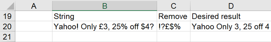
Imagine you have a set of text strings and want to specify which characters should be removed from those strings dynamically:

Liam Bastick’s article from 2020 briefly touches on how to do this with a recursive LAMBDA, but here we’ll explore the ideas in a bit more detail. The purpose of this article is how to place a complex formula inside a LAMBDA name to get an easily usable user-defined function.

The core idea is to convert the string in col. B to an array of characters; for each character, if it is in the string of characters to be removed, change it to a null string, otherwise leave it unchanged; and finally concatenate the array of remaining characters to the result.

To convert a string to an array, use the MID() function with a SEQUENCE() dynamic array function to produce an array of characters.

The function = SEQUENCE(LEN(B20)) returns an array of as many index numbers as characters in B20, in this example 27:

={1;2;3;...;27}

Using MID around this returns an array of characters

=MID( B20, SEQUENCE( LEN( B20)), 1)

We can use the SEARCH function to test for each of these being present in C20: 

=SEARCH( MID( B20, SEQUENCE( LEN( B20)), 1), C20)

The return array elements are either a number (found) or #VALUE! (not found):

={#VALUE!;#VALUE!;#VALUE!;#VALUE!;#VALUE!;1;#VALUE!;...;4;#VALUE!;1}

We put that formula inside IF and ISERROR (to return either the original character (if error) or null (if not error):

=IF( ISERROR( SEARCH( MID( B20 , SEQUENCE( LEN( B20)), 1) ,C20)), MID( B20, SEQUENCE( LEN( B20)), 1) ,"")

={"Y";"a";"h";"o";"o";"";" ";"O";"n";"l";"y";" ";"";"3";",";" ";"2";"5";"";" ";"o";"f";"f";" ";"";"4";""}

Finally, we concatenate that to the desired result

=CONCAT( IF( ISERROR( SEARCH( MID( B20, SEQUENCE( LEN( B20)), 1), C20)), MID( B20, SEQUENCE( LEN( B20)),1),""))

Which gives us:

Yahoo Only 3, 25 off 4

You will notice the repeated MID() subexpression. We can simplify that by using LET to create a temporary name 'aChar':

=CONCAT( LET( aChar, MID( B20, SEQUENCE( LEN( B20)), 1), IF( ISERROR( SEARCH( aChar, C20)), aChar, "")))

And now we can make this a nice user-defined function by making B20 and C20 parameters of a LAMBDA name 'RemoveCharacters'

RemoveCharacters =LAMBDA( text, remove, CONCAT( LET( aChar, MID( text, SEQUENCE( LEN( text)), 1), IF( ISERROR( SEARCH( aChar, remove)), aChar, ""))))

=RemoveCharacters(B20,C20)

Yahoo Only 3, 25 off 4

Slugify

To use recursion to ‘slugify’ text means to lowercase the text, remove all special characters leaving only numbers and alphabetic characters, and separate words by dashes instead of spaces.

This is very common in URLs which cannot handle special characters. For example, "Yahoo! Only £3, 25% off $4?" becomes "yahoo-only-3-25-off-4"

To achieve this there are multiple steps required: convert the text to lowercase; then to an array of characters; convert non-alphanumeric characters to spaces; concatenate the resulting array; reduce multiple spaces to single spaces; and finally change all spaces to dashes.

To test for a character being in the wanted range, we want to accept it if EITHER it is >="0" AND <="9", OR it is >="a" AND <="z"

We cannot use the Excel AND() and OR() functions in a dynamic array formula as they do not accept arrays. But we use Boolean formulas and multiplication/addition to give the effect of AND and OR respectively – something that we covered when looking at the FILTER function in Tip #443.

So, ( ch>="0" ) * ( ch<="9") returns 1 if both are true, otherwise 0, and ( ch>="0" ) + ( ch<="9") returns non-zero (true) if either is true, otherwise 0.

This function will produce the first result:

=CONCAT( LET( ch, MID( LOWER (B20), SEQUENCE( LEN( B20)),1), IF((ch>="0")*(ch<="9")+(ch>="a")*(ch<="z"), ch, " ")))

yahoo  only  3  25  off  4

and we then use TRIM() to reduce multiple spaces to one space, and SUBSTITUTE to change spaces to dashes:

=SUBSTITUTE( TRIM( CONCAT( LET( ch,MID( LOWER( B20), SEQUENCE( LEN( B20)), 1), IF((ch>="0")*(ch<="9")+(ch>="a")*(ch<="z"), ch," ")))), " ", "-")

yahoo-only-3-25-off-4

To make that complex formula available as a simple UDF, convert it to a LAMBDA

Slugify =LAMBDA( text, SUBSTITUTE( TRIM( CONCAT( LET( ch, MID( LOWER( text), SEQUENCE( LEN( text)), 1), IF((ch>="0")*(ch<="9")+(ch>="a")*(ch<="z"), ch," ")))), " ", "-"))

=Slugify(B20)

yahoo-only-3-25-off-4