Yes or no. True or false. Right or wrong. The humble ‘check’ or ‘tick’ mark has been an effective way to denote acceptance for centuries. And, of course, it has existed in Excel for quite a long time too, but only as a Form Control. This has caused headaches for Excel users, and while our webinar last year highlighted that they were relatively simple to set up, they are not without limitations and ultimately it can be tricky to deliver a seamless user experience with them. Also, because they are rooted in the world of VBA, users opening workbooks in Excel Online would be unable to use them.

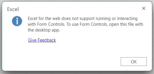
The good news is that finally, Excel has introduced Checkboxes as a feature that sits inside cells. The feature has rolled out to all users in Microsoft 365 Current Channel so if you’ve got all your updates downloaded, you should have the option to add them to your workbook. And yes, it’s available in Excel Online too, as well as Macs, and is coming to mobile devices too.

Setup and basic interaction

Adding Checkboxes to your workbook is as simple as selecting the cell(s) you want to add them to, and going to Insert > Checkbox.

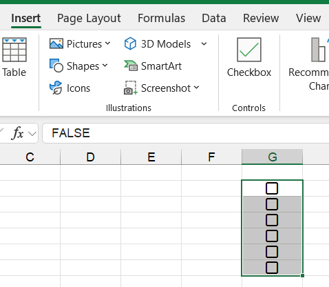
You’ll see from the screenshot that in the formula bar the contents of the cell when the box is unticked shows as FALSE, which is the default state. Logically, when the box is ticked (which you change by clicking on it, or selecting the cell and hitting the space bar), it changes to TRUE.* This also means that if you already have a column with a TRUE/FALSE flag, you can select the cells and Insert>Checkbox will turn them into checkboxes with the true cells all ticked, although this won’t work if you use other flags like T/F, Y/N or 1/0.

There are some quirks when working with checkboxes, which are in part due to their slightly awkward position somewhere between cell formatting and cell content. If you select a ticked cell and press the delete key, it clears the tick. It requires pressing the delete key twice to delete the checkbox entirely, but only if one or more of the selected checkboxes has a tick in it.

Meanwhile, going to the ‘Clear’ option on the Home tab (the rubber in the Editing section) also turns up some curious behaviour – clear formats turns the checkboxes back to TRUE/FALSE flags, while clear contents works the same as the delete key.

* Some have argued that checkboxes should have three states – true, false and blank or null – however the practicalities of this would have made them a much more complex feature to implement and use.

Using checkboxes as an input

The most common use case for checkboxes is likely to be some sort of flag on a data table. Because the checkboxes are essentially formatted cells sitting over a TRUE/FALSE flag, this makes it very easy to use them in formulas or conditional formatting.

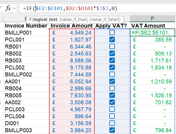
For example, to use checkboxes as part of an IF or FILTER function, it is only necessary to reference the cell or range because the checkbox inherently returns the true or false value that the function is expecting. Take this example of a list of invoices – using checkboxes for a simple VAT flag, it is then possible to set up an IF statement where the logical test is simply the value of the checkbox column, returning the calculated VAT if the box is ticked, and zero if it isn’t.

Similarly, checkboxes can be used to support conditional formatting. To highlight a row where a checkbox is ticked, select the data table you want the formatting to apply to, go to Home>Conditional Formatting>New Rule…, select “Use a formula to determine which cells to format”, and in the formula bar specify just the checkbox cell.

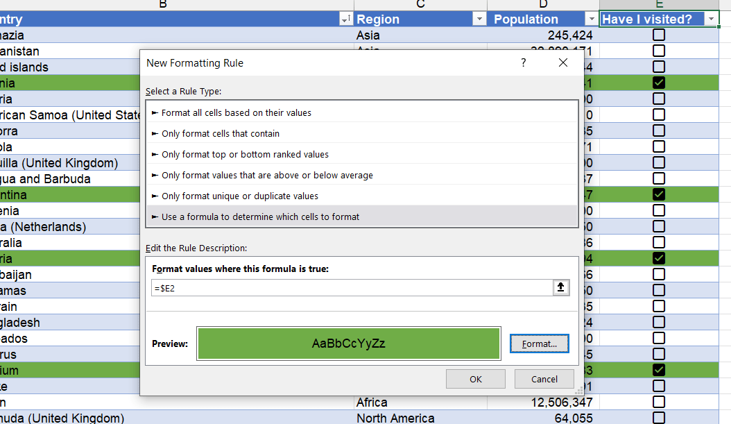
Note, this is the correct way to reference cells when applying conditional formatting to an entire table, with the $ symbol before the column, and the row number being the first row of the table – something we covered way back in Tip #143.

Formula-driven checkboxes

Further digging into the murky world of whether a checkbox is cell formatting or cell contents, it is actually possible to set up a formula that returns a TRUE/FALSE flag, and then this can be turned into a checkbox.

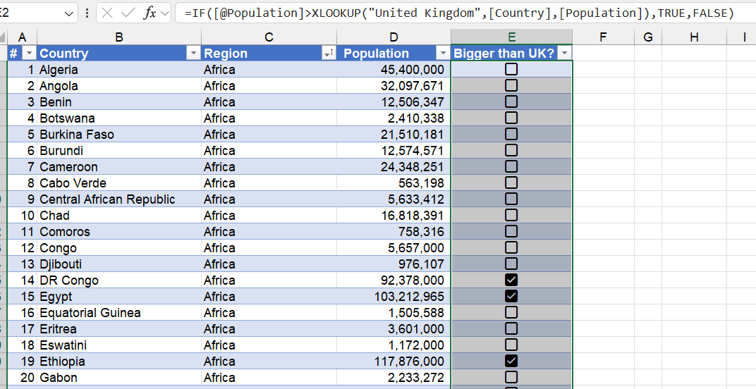
Say, in a table list of countries I want to flag the countries that have a larger population than the UK, I would set up the following function:

=IF([@Population]>XLOOKUP("United Kingdom",[Country],[Population]) ,TRUE,FALSE)

We can then select the flag column and go to Insert > Checkboxes, and it turns the formula-driven TRUE/FALSE flag to checked and unchecked boxes, which then update based on any changes to the condition.

Just to check…

It’s worth noting that Google Sheets has had this functionality for years (and called them “tick boxes” – a tip of the cap to the use of British English, thanks Google!), and perhaps unsurprisingly, Excel’s version is basically identical. In Google Sheets you can find tick boxes on the Insert menu. Unfortunately, when you download a Google Sheet with tick boxes as an Excel file, it will just display them as TRUE/FALSE; the same is true in reverse, so the compatibility between Excel checks and Google ticks isn’t quite there yet.

It’s also curious to note that currently the Checkbox option sits in its own group on the ‘Insert’ tab. ‘Controls’ would imply more than one – could we see some additional features sitting here in the not too distant future? Certainly, combo boxes, list boxes and option buttons would all be popular Form Controls to add as native features – do you have any others you’d like to see?