Adding calculated fields to the GROUPBY function

There is an obvious comparison to make between PivotTables and the new GROUPBY and PIVOTBY functions. They both summarize data into a tabular form. But there are also many differences which gives each its strengths.

One feature of PivotTables that many advanced users utilize is calculated fields. These are additional calculations based on the values already contained within the PivotTable.

GROUPBY and PIVOTBY, by themselves, do not have a calculated field feature. However, we can extend their native capabilities by using other functions.

Recap on PivotTable Calculate Fields

Before we dive into the formula solutions, let’s remind ourselves about how calculated fields work.

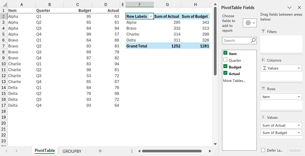
From the data in A2:D17 we’ve created a PivotTable containing:

• Rows: Item
• Values: Actual, Budget (Excel automatically applied a SUM calculation)

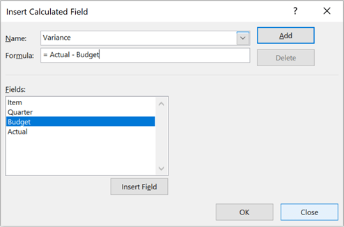
To calculate the variance and % variance for each Item we can use calculated fields.

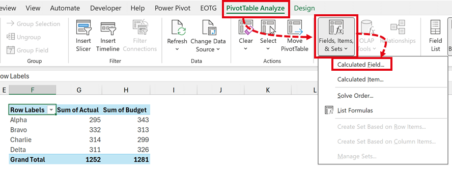
To add a calculated field, select a cell in the PivotTable and click PivotTable Analyze > Fields, Items & Sets > Calculated Field... from the ribbon.

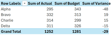
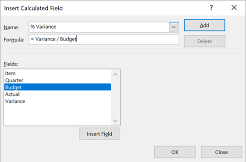
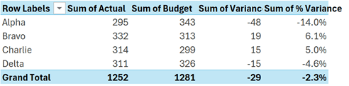
While the automatically created name is Sum of % Variance, this is misleading. It does not perform a sum. The calculation is based on the existing results in the PivotTable.
Overall, I think we can agree that calculated fields are a really helpful feature.

GROUPBY Calculated Fields

Let’s now turn our attention to GROUPBY.

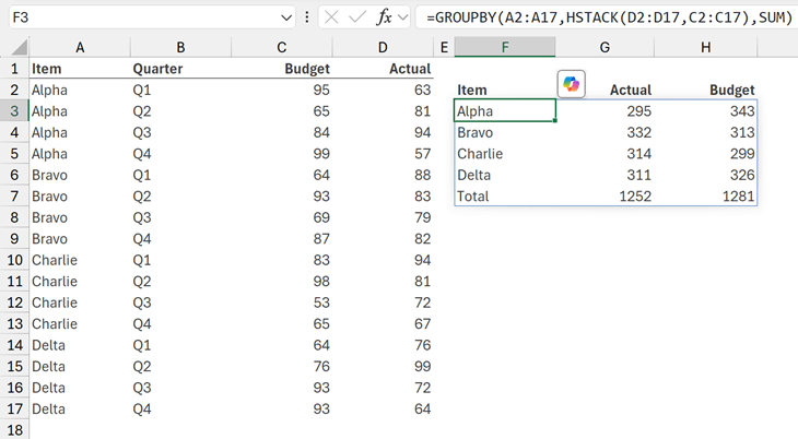
Using the same data, the formula in cell F3 is:

=GROUPBY(A2:A17,HSTACK(D2:D17,C2:C17),SUM)

• A1:A17 are the row fields which appear on the left.
• HSTACK(D1:D17,C1:C17) are the values to calculate on. HSTACK puts the ranges into the order of Actual, then Budget.
• SUM is the calculation to perform on each value column.

The column headers in F2:H2 are entered directly into the cells.

This displays the same result as our original PivotTable. Now it’s time to add our additional calculations.

Calculating the Variance

For the variance calculation we are performing a SUM, therefore we can either:

Method #1: Calculate the variance between Actual and Budget for each row and sum the values.

Method #2: Sum the Actual and Budget values then calculate the variance of the results.

Both methods return the same result.

Method #1

To calculate the variance between Actual and Budget on a row-by-row basis, we can add the calculation into the GROUPBY function.

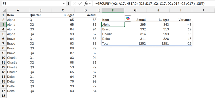
The formula in cell F3 is:

=GROUPBY(A2:A17,HSTACK(D2:D17,C2:C17,D2:D17-C2:C17),SUM)

As shown by the bold values. the variance is calculated row by row, then SUM aggregates all the values.

The method may seem easy, however we can’t use it to calculate the % variance (which we will see shortly). So, we may decide to use Method #2 instead.

Method #2

The second method for calculating the variance is to use the result from the GROUPBY in the subsequent calculation.

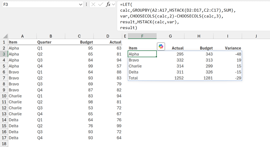
The formula in cell F3 is:

=LET(
calc,GROUPBY(A2:A17,HSTACK(D2:D17,C2:C17),SUM),
var,CHOOSECOLS(calc,2)-CHOOSECOLS(calc,3),
result,HSTACK(calc,var),
result)

• LET allows us to allocate names to interim calcuations which are used later in the formula. We have created 3 names: calc, var and result.
• calc,GROUPBY(A2:A17,HSTACK(D2:D17,C2:C17),SUM) – this is the previous GROUPBY calculation allocated to the name calc.
• var,CHOOSECOLS(calc,2)-CHOOSECOLS(calc,3) – the performs the calculation of column 2 from the GROUPBY (which is Actual) less column 3 from the GROUPBY (which is Budget). This value is allocated to the name var.
• result,HSTACK(calc,var) – the combines the calc and var into a single array called result.
• result - the last argument in LET is the value to return. We want to return the result name.

This method is longer and may initially appear more confusing. However, the methodology of calculating based on existing results is the same approach used by PivotTable calculated fields.

Calculating % Variance

The percentage variance needs to be calculated on the result of the GROUPBY. Therefore, by extending Method #2, we can easily incorporate this calculation.

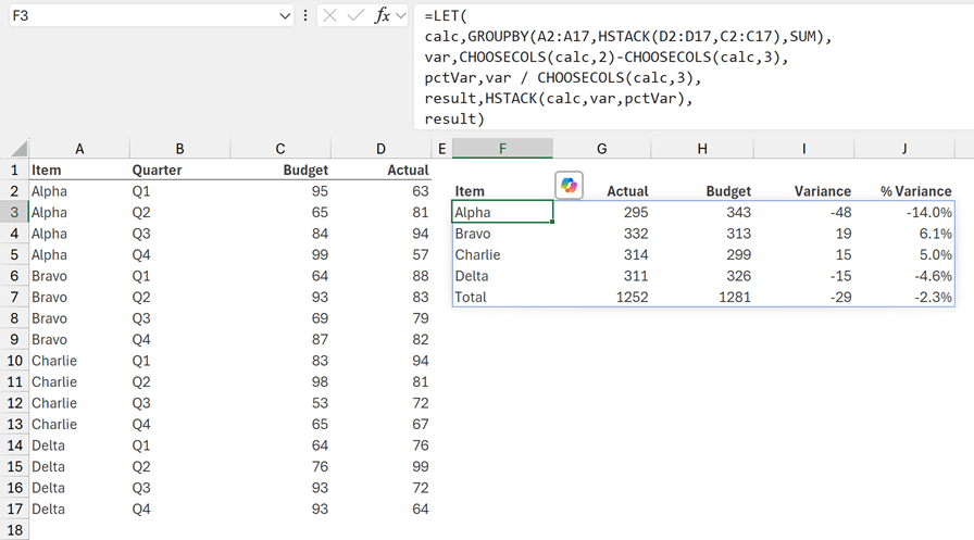
The formula in cell F3 is:

=LET(
calc,GROUPBY(A2:A17,HSTACK(D2:D17,C2:C17),SUM),
var,CHOOSECOLS(calc,2)-CHOOSECOLS(calc,3),
pctVar,var / CHOOSECOLS(calc,3),
result,HSTACK(calc,var,pctVar),
result)

The formula above is the same as Method #2 with the additions marked in bold:

• pctVar,var / CHOOSECOLS(calc,3) – this calculates the % variance using the previous var calculation divided by the column 3 of the GROUPBY (which is the Budget). This result is allocated to the name pctVar.
• result,HSTACK(calc,var,pctVar) - the pctVar is combined into the final result.

Using this formula, we have replicated the calculated fields functionality. Using this methodology, we can add as many calculations as we wish; including calculations which are not possible with PivotTables.

Calculating Text

Standard PivotTables do not calculate text. Therefore, this example illustrates the benefits of using GROUPBY. Let’s suggest we want to add a text value of Good, OK or Bad to describe the % variance.

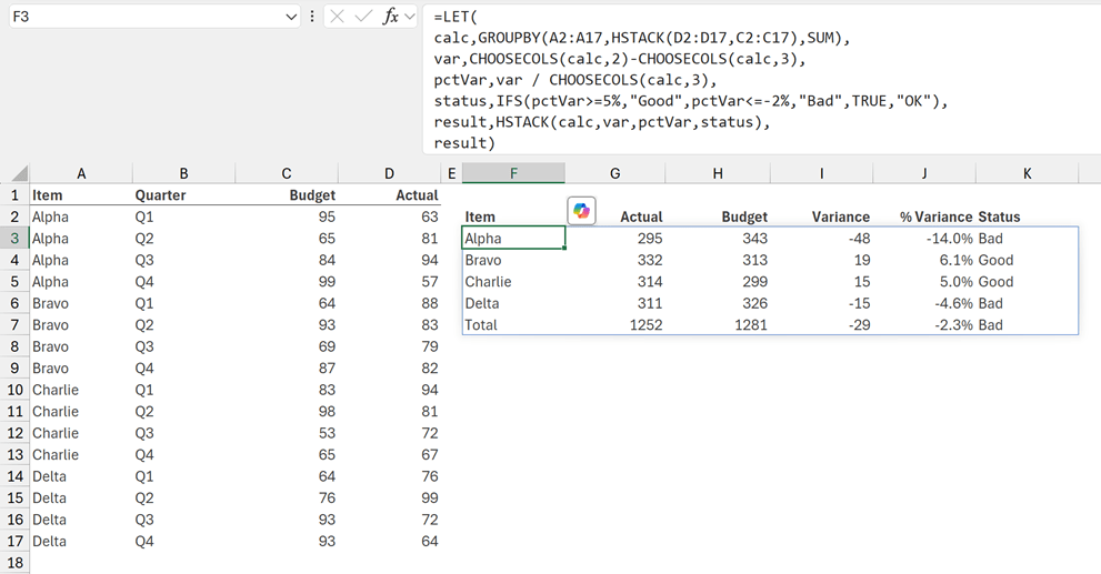
The formula in cell F3 is:

=LET(
calc,GROUPBY(A2:A17,HSTACK(D2:D17,C2:C17),SUM),
var,CHOOSECOLS(calc,2)-CHOOSECOLS(calc,3),
pctVar,var / CHOOSECOLS(calc,3),
status,IFS(pctVar>=5%,"Good",pctVar<=-2%,"Bad",TRUE,"OK"),
result,HSTACK(calc,var,pctVar,status),
result)

The changes marked in bold are:

• status,IFS(pctVar>=5%,"Good",pctVar<=-2%,"Bad",TRUE,"OK") – this calculates the word Good, Bad or OK depending on the % variance, and allocates the values to the name of status.
• result,HSTACK(calc,var,pctVar,status) - the status is incorporated into the final result.

Using this formula, we have replicated the calculated fields functionality. Using this methodology, we can add as many calculations as we wish; including calculations which are not possible with PivotTables.

Conclusion

In this article, we have seen how to apply the concept of PivotTable Calculated Fields to the GROUPBY function. Using LET, we can create interim calculations that can be combined into the final result using HSTACK.

And through this approach, we have seen that GROUPBY, while requiring more skill, can produce results which are not possible with standard PivotTables.