Aligning data in PowerQuery

The question

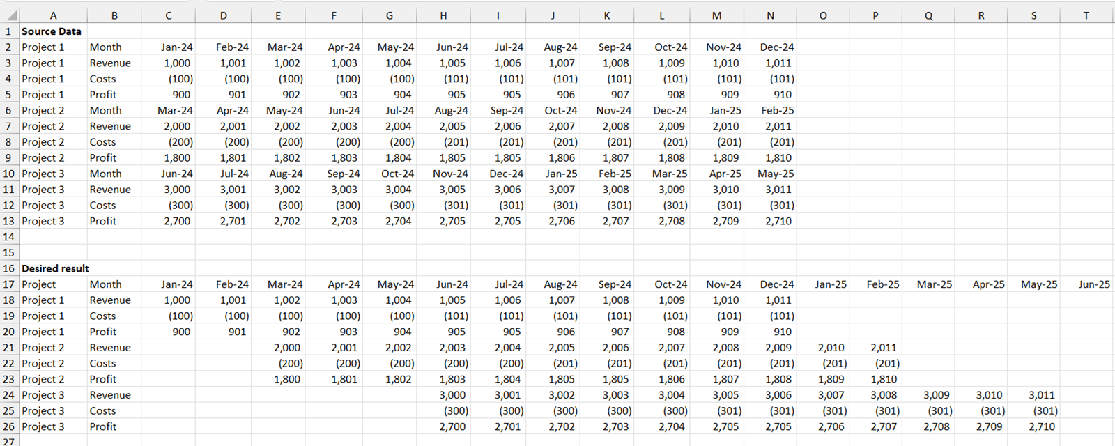
Imagine you have data from several sources, where the row labels are the same, but the periods differ. For example, the "first column of data" might represent Jan-24 in the first file, but the first column in the second file represents Mar-24, and a third file starts with Jun-24. How can you align the data so that the columns are consistent across months? In this article, we will explore how to do this using PowerQuery in a way which can automatically accommodate additional line items, projects and periods.

This article is intended as a Creator-level tutorial and assumes a basic familiarity with PowerQuery and Pivot tables. Download links for the example ‘starting’ and ‘ending’ files can be found at the end of this article.

The complication

The problem could be solved on the example data by splitting the source data into 3x individual tables, one for each project, and then unpivoting them separately before appending back together. The issue with that that technique is that it is not scalable for additional projects without more work in PowerQuery to add the extra interim tables for each project. This article will cover a solution which can be scaled for more projects, periods and P&L lines!

The idea

The overall idea is that we need to label the data points with their corresponding period, and the corresponding period will depend not only on which column the data was in but also which project, as each column could relate to a different period depending on which project the data was from. So, we need to first make a lookup table which will map columns to dates, depending on which project it was, and unpivot the data points themselves whilst keeping track of which column and project they were from so that we can map on the periods from the lookup table.

The broad steps are therefore as follows:

1. Load the source data into PowerQuery.
2. Create a Headings table – this will contain a list of projects record which month each column related to. Then add a “key” field.
3. Create a Data Table – this will contain the actual data. It needs to be unpivoted and then have a similar “key” field added to record which column and project each data item relates to.
4. Map the dates from the Headings table to the Data table using the Key.
5. Finalise the data by deleting all interim helper columns, and load the data into a PivotTable on the grid.

This guide will take you step-by-step through the process in PowerQuery.

Step 1 – load the source data into PowerQuery

The source data is not yet formatted as a table. We will first convert the range to a table object, so that it can be expanded later, then it needs to be loaded to PowerQuery.

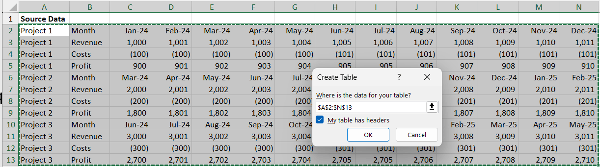
1. Convert the range to a Table object.
   (Highlight the table. Click on “Insert > Table”. Leave “My table has headers” ticked. Click on “OK”.)

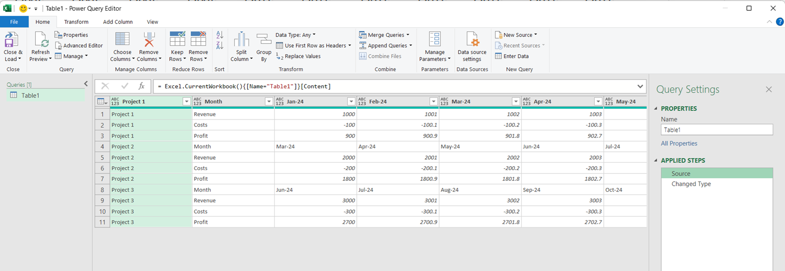
2. Load the table to PowerQuery.
   (Click on the table. Then navigate to “Data > From Table/Range”. PowerQuery will open with a new query relating to the data from your table.)

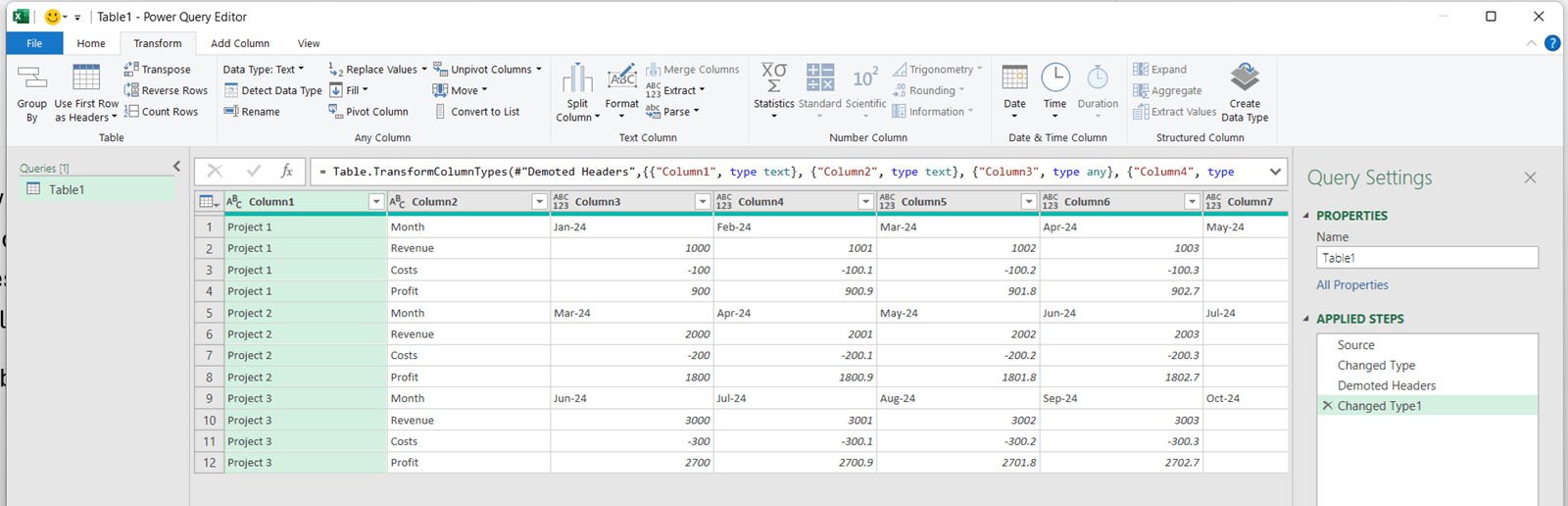
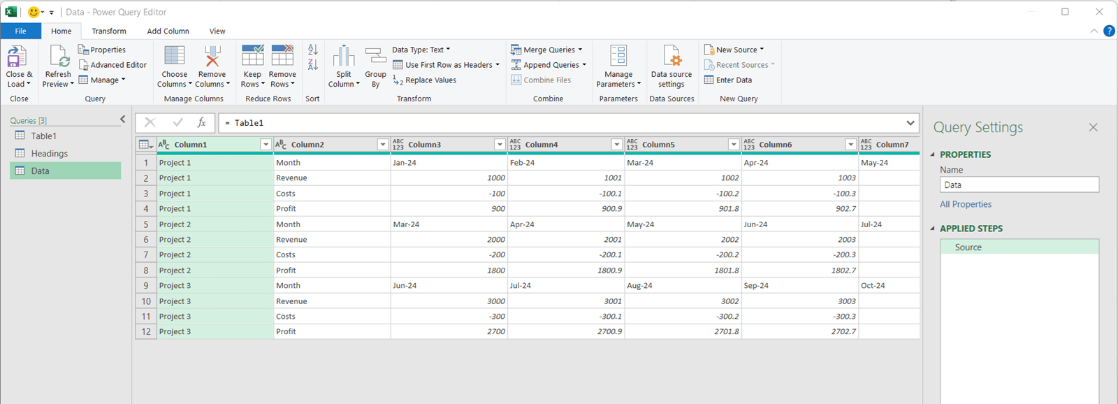
3. Demote the headings to the first row of data.
   (Click on “Transform > Use First Row as Headers > Use Headers as First Row”.)

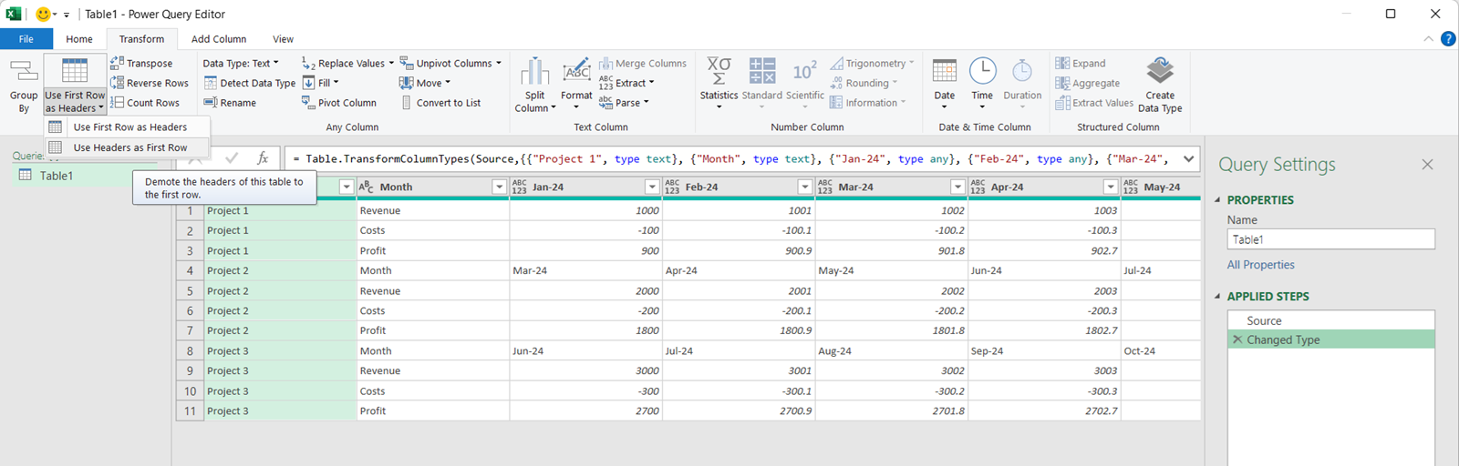
4. This is the result:

Step 2 – create a Headings table

This will contain a list of projects and columns and record which months they related to, and then add a “key” field.

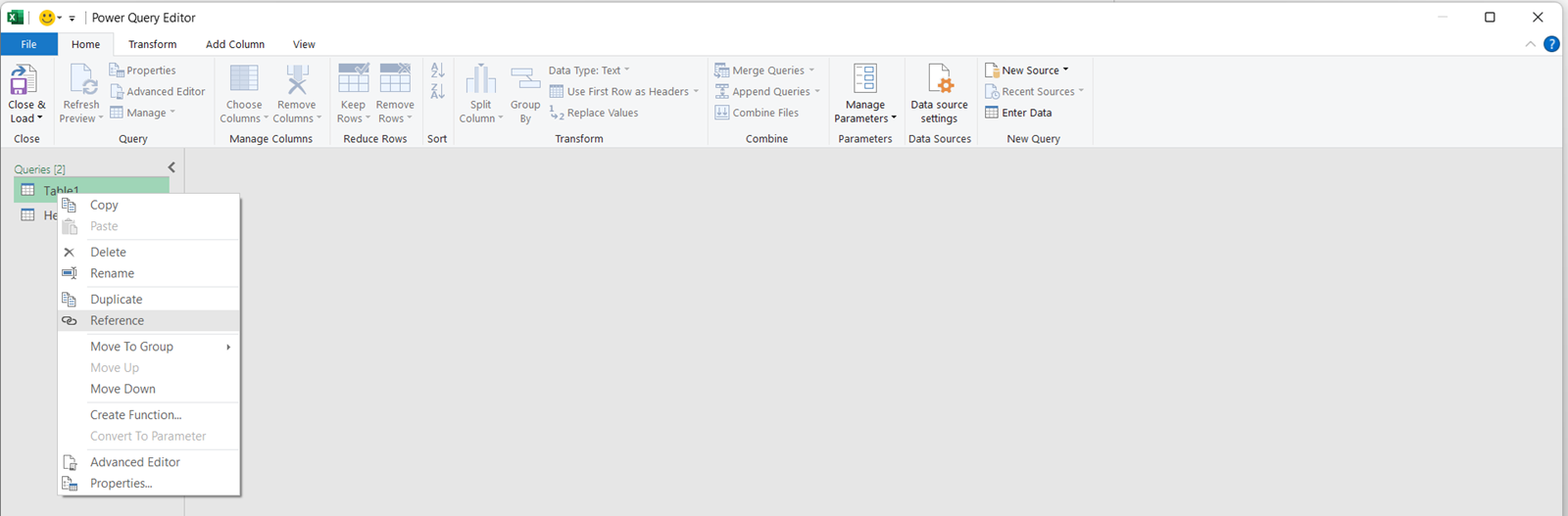
1. Create a new table, which references Table 1 as its source.
   (Within the editor, right click on “Table1”, then click on “Reference”.)

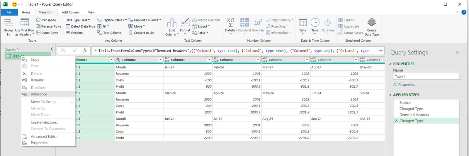
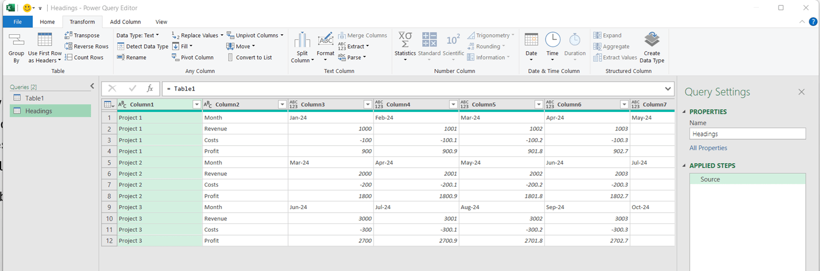
2. Rename the new table as “Headings”.
   (Double click on the table name and type “Headings”.)

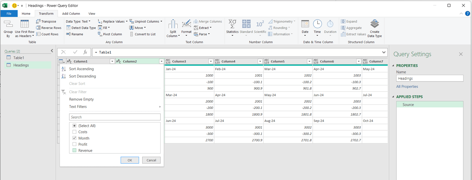
3. Filter to only keep the heading rows, which are identified as having the value “Month” in column 2.
   (Click on the arrow on the column 2. Select only the values of “Month” from the drop-down list and click “OK”.)

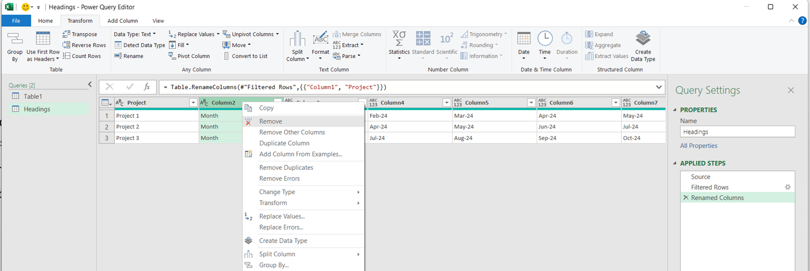
4. Rename “Column 1” as “Project” and remove “Column 2” as it's no longer needed.
   (Double click on the title of column 1 and rename. Then right click on column 2 and select “Remove”.)

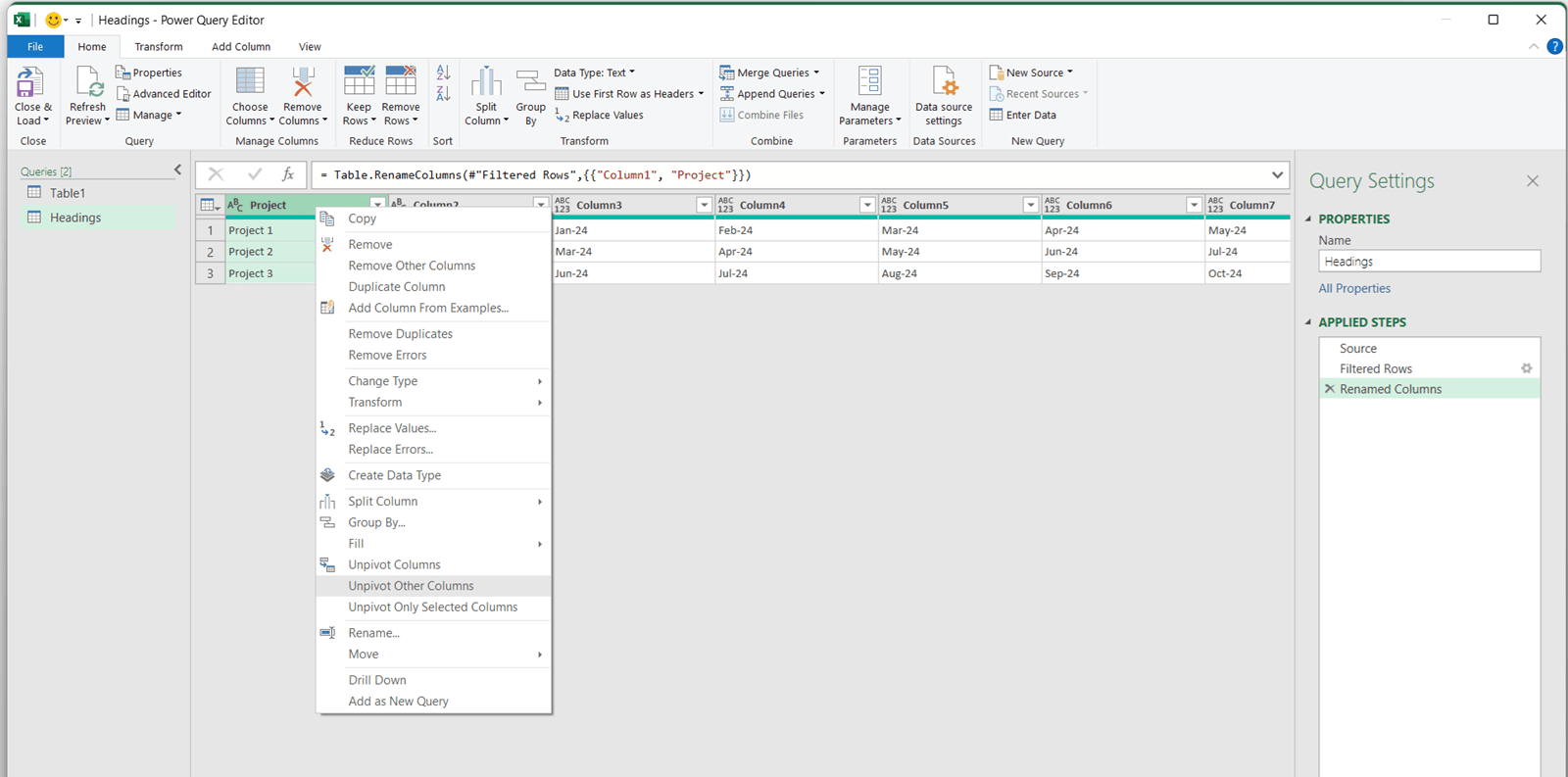
5. Unpivot by all columns, other than “Project”.
   (Right click on the “Project” column and click on “Unpivot other columns”.)

6. Rename the “Attribute” column as “Col”.
   (Double click on the heading “Attribute” and type “Col”.)

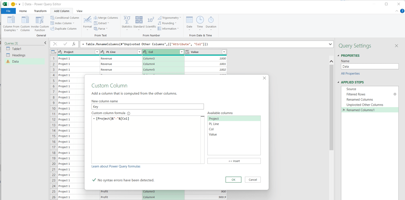
7. Create the unique Key field, being the concatenation of Project and Col.
   (Click on “Add Column > Custom Column” and then name it as “Key”. Write the following custom formula:

   = [Project]&"-"&[Col]

   and click “OK”.)

    

It is noted that creating a Key field is not strictly required. An alternative approach would be to select both Project and Col fields during the later “Merge Queries” step. However the Key field technique is used in this article for clarity, and to demonstrate how to create a simple custom column.

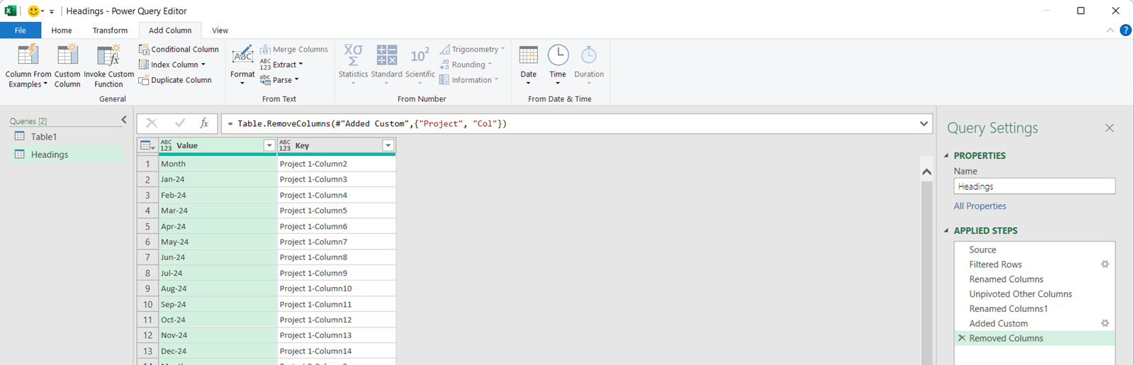
8. Remove the “Col” and “Project” columns to leave the following:
   (Right click on each column and click on “Remove”.)

Step 3 – create the Data table

This will contain all the individual data points, along with the project and P&L line label they relate to, as well as the column they originally came from – plus a new “key” field will be added ready to map on the actual dates themselves.

1. Create another new table, which references Table 1 as its source.
   (Within the editor, right click on “Table1” and click on “Reference”.)

2. Rename the new table as “Data”.
   (Double click on the table name and type “Data”.)

3. Filter to only keep the data rows, as identified as NOT having the value “Month” in column 2.
   (Click on the arrow on the column 2 and choose “text filter”. Then enter a new rule to “Keep rows where column 2” “does not equal”, and enter “Month” in the final field. Note: we use this method in case other fields are added to the source data later.)

It is noted that PowerQuery may automatically create the rule as “does not equal” if you only uncheck a single item from the drop down list. However, the method described here is explicit.

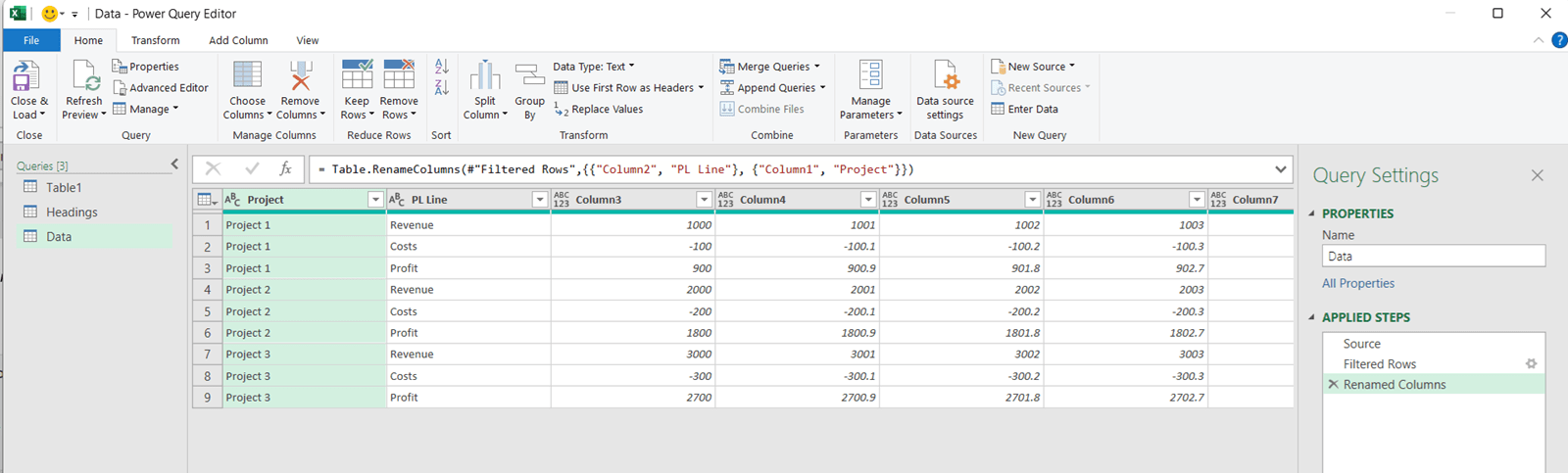
4. Rename column 1 as “Project” and column 2 as “PL Line”.
   (Double click on each column title and type “Project” and “PL Line”.)

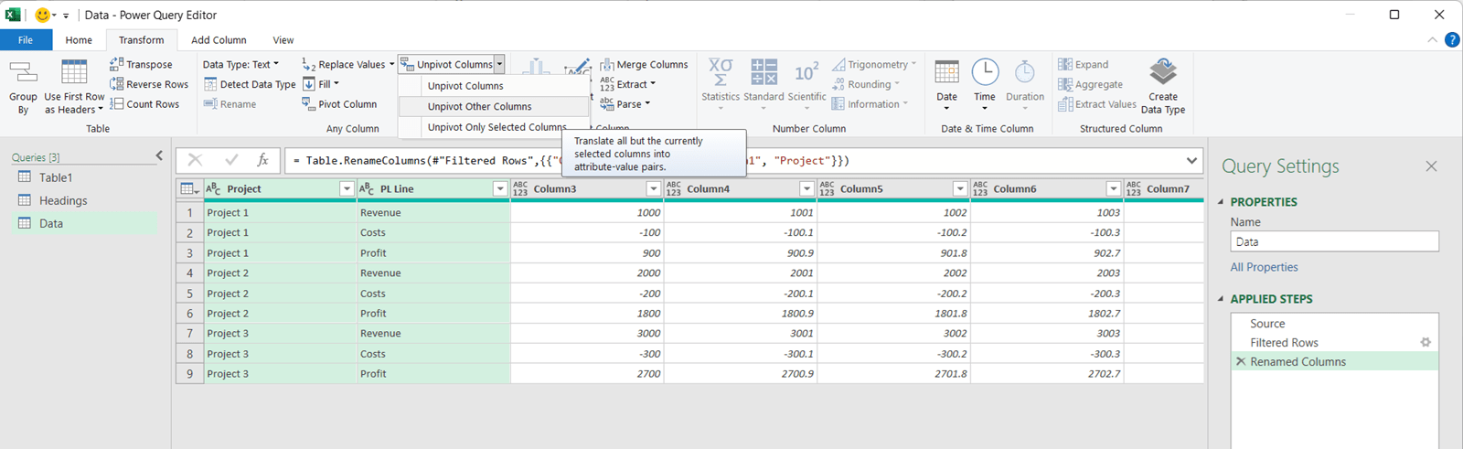
5. Unpivot by all columns, other than “Project” and “PL Line”.
   (Use CTRL and click on “Project” and “PL Line” columns so they are both green, ie, selected. Then click on “Transform > Unpivot Columns > Unpivot other columns”.)

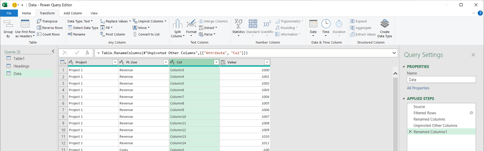
6. Rename the Attribute column as “Col”.
   (Double click on the “Attribute” column heading and type “Col”.)

7. Create the unique “Key” field, being the concatenation of “Project” and “Col”.
   (Click on “Add Column > Custom Column” and then name it as “Key”. Write the following as the custom formula:

   = [Project]&"-"&[Col]

   and click “OK”. Alternatively, click on the names of “Project” within the available columns. Click “Insert” then type in &”-“& and then click on the name of “Col” field. Click “Insert” to finish the formula, and click “OK”.)

    

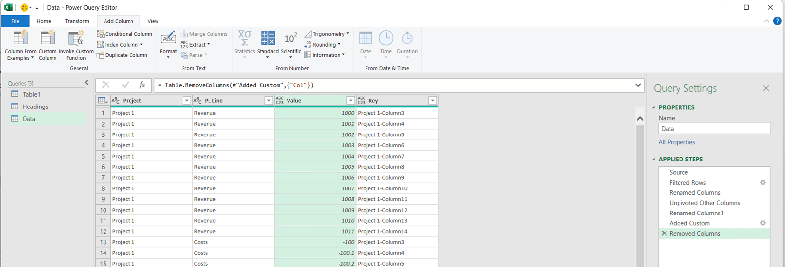
8. Remove the “Col” column to leave the following:
   (Right click and click on “Remove”.)

Step 4 – map the dates from the Headings table to the Data table

Now we can combine the queries and map on the actual dates to the data, using the Key field which is present on both tables.

1. With the “Data” query selected, click “Home > Combine > Merge Queries”.

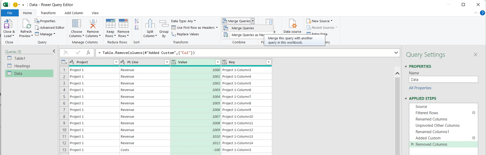
2. The first table should be the “Data” query.
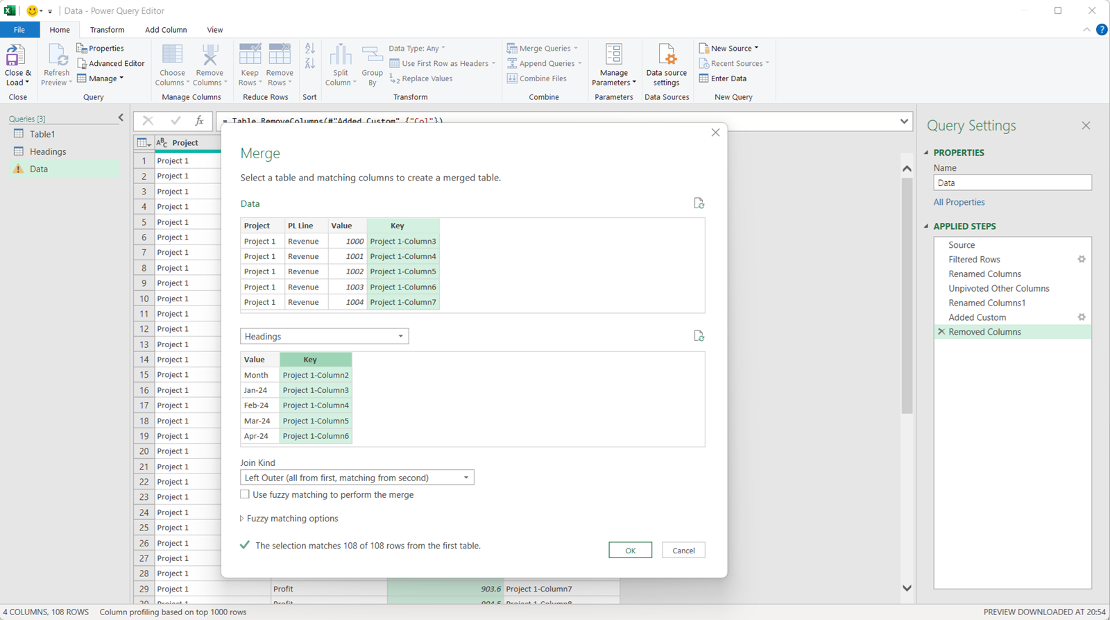
   (Select the “Key” column. Choose the second table as the “Headings” query, and select the “Key” column from there. Click OK.)

Make sure to use default join kind “Outer Left”, not to use fuzzy matching. There should be a 100% match. See 108/108 rows are matched in this example.)

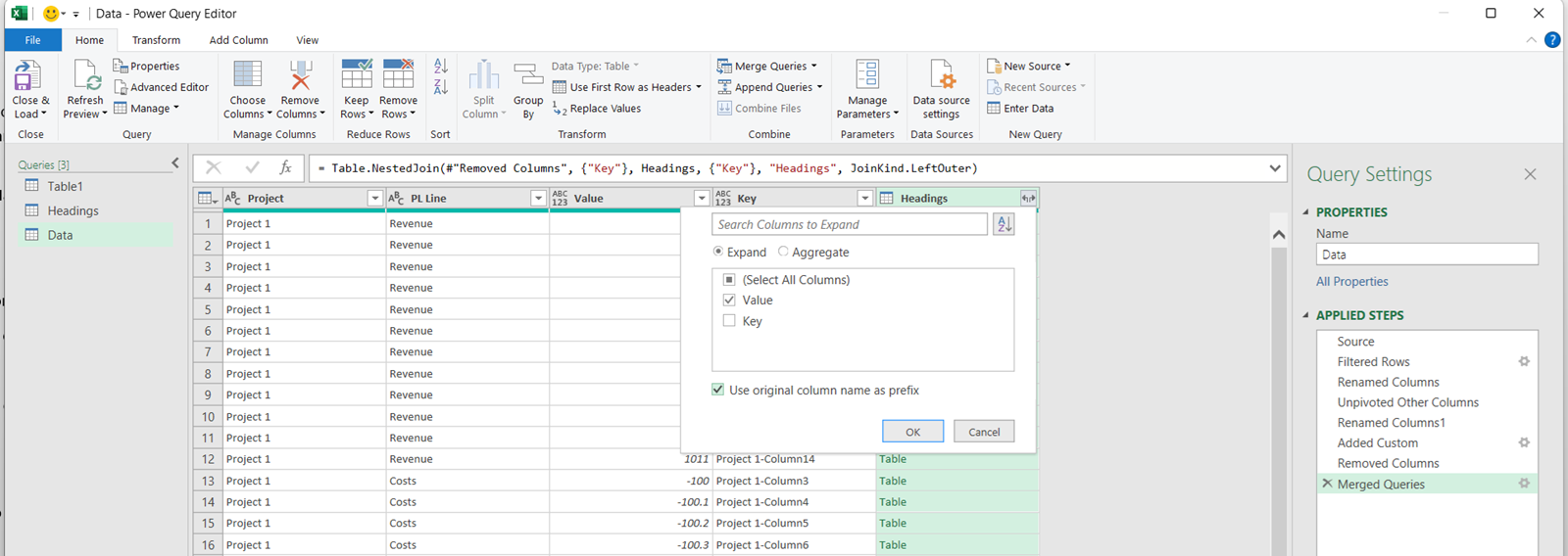
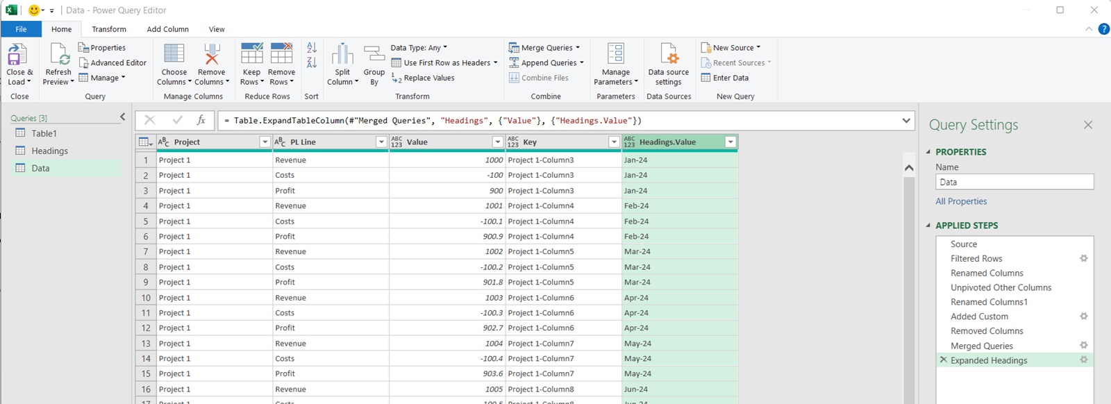
3. Keep only the “Value” field from the Headings table.
   (Click on the “opening arrows” next to the "Headings" field header. Then select “Value” from the list. Leave “Use original column name as prefix” ticked.)

4. All rows now have a value, a project number, and the date which we have mapped on. This is the current state of the data:

Step 5 – finalise the data

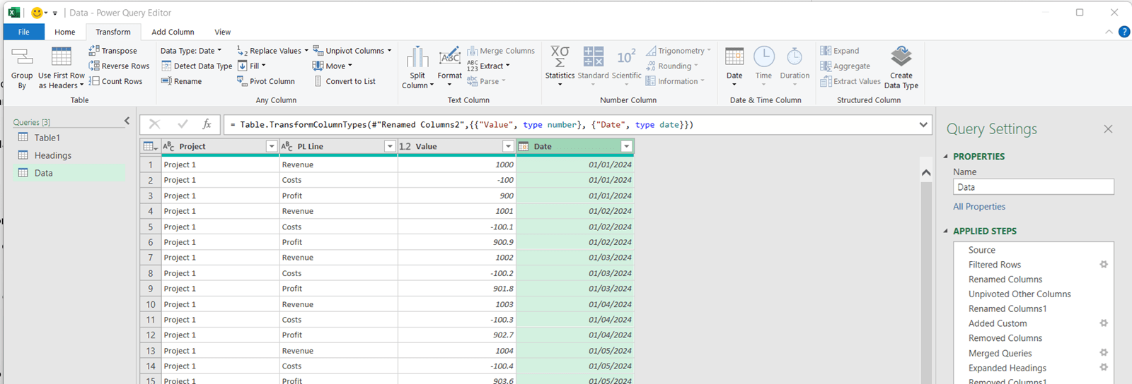
1. Remove the Key column.
   (Right click on the column heading and click on “Remove”.)
2. Rename the “Headings.Value” column as “Date”.
   (Double click on the column title and type “Date”.)
3. Change the “Value” field to a decimal number, and the “Date” field to a date.
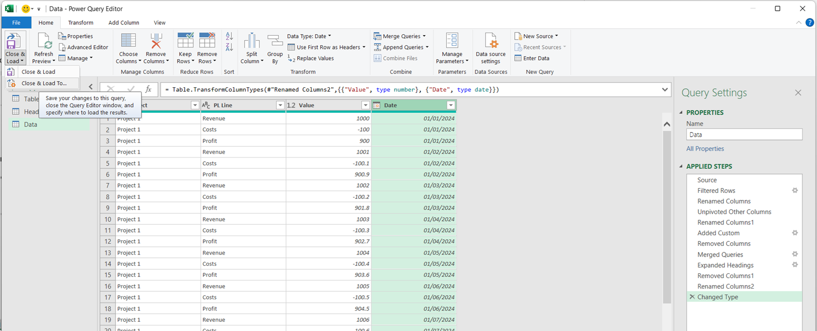
   (Click on each column, then under “Transform” tab. Click on the “Data type” drop down and select the appropriate type.)
4. This is the final resulting data:

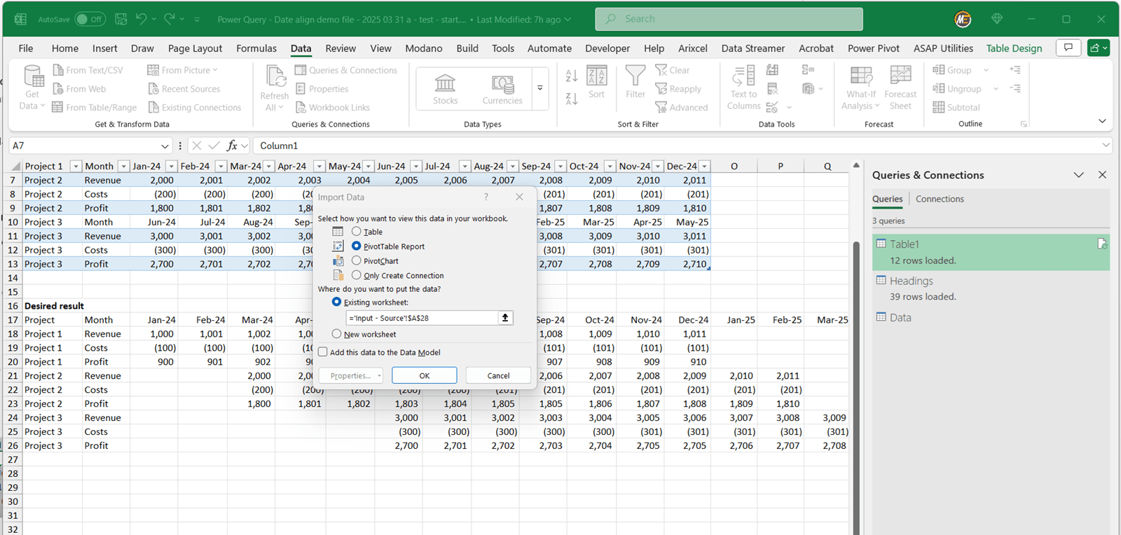
5. The last step is to load it onto the grid as a PivotTable and customise it.
   (With the data table selected, click on “Home”. Click on the arrow under “Close and load” and select “Close and Load to”.)

6. Load the data to a PivotTable underneath the “desired result”.
   (Click on “PivotTable report”, “Existing worksheet”, and then use the range selection tool to choose cell A28, and click “OK”.)

7. Customise the PivotTable to add “Project Value” and “PL Line” into the “Rows” section, “Dates” across the top, and values in the “Values” section.
   (Drag each field from the PivotTable field list into the corresponding section on the pane on the right-hand side of the Excel window. If “Years” and “Quarters” are added automatically, untick them to leave only “Months”.)

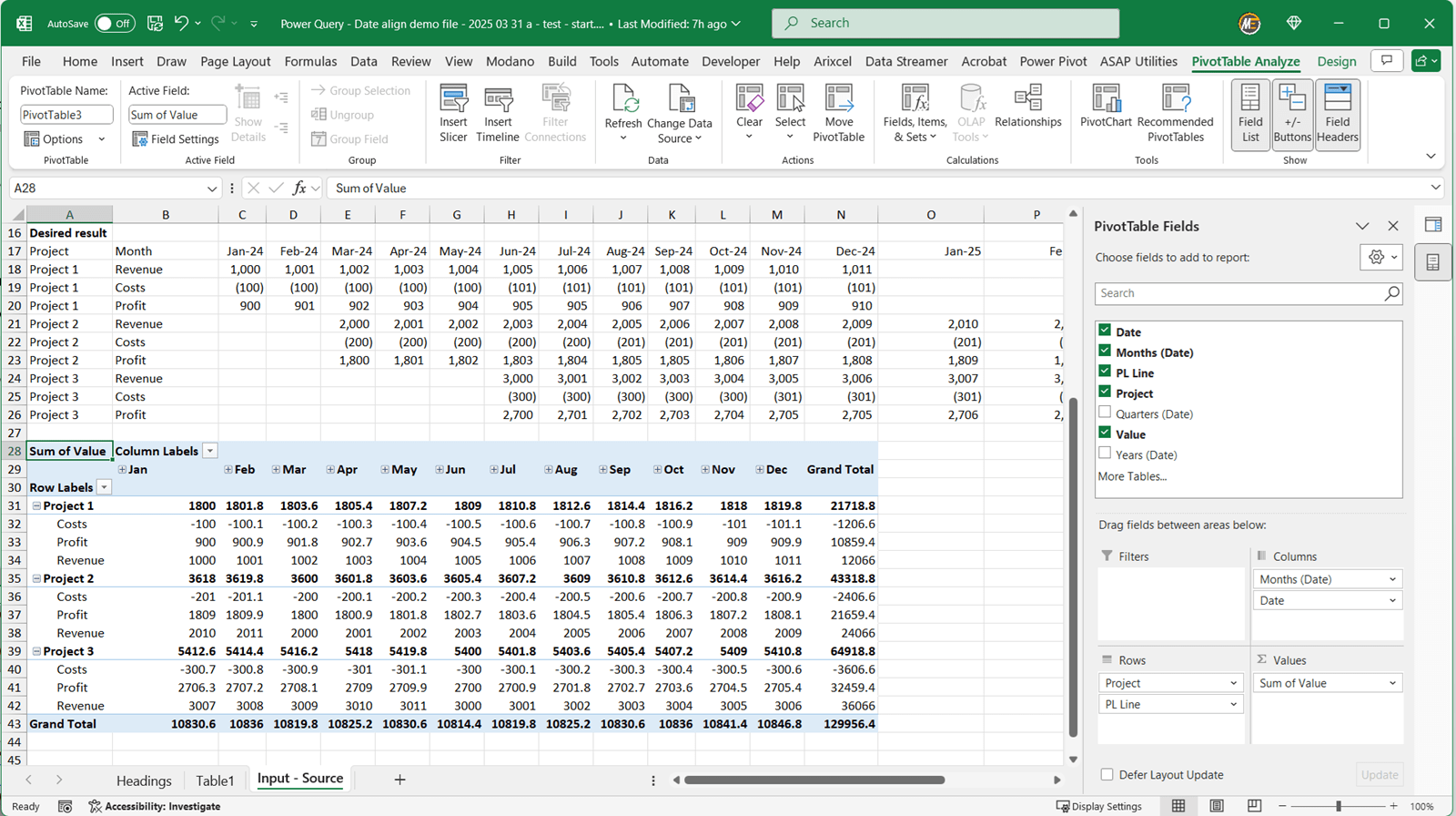
The report data now matches the desired result!

(There will be a little more work involved in customising the format of the PivotTable into a presentable report – eg formatting the numbers and ordering the PL Lines – but that is outside the scope of this article.)

Conclusion

Even when data doesn't align across sources, it isn't too difficult to align the columns, once you understand how! The key is creating an interim “Headings” table to map column positions against the respective dates, allowing the date mapping to vary by division by concatenating the Project and Column.

This article includes download links for the example ‘starting’ and ‘ending’ files, so why not give it a try and put your PowerQuery skills to the test to see if you can re-create the outcome?

Hopefully, this guide has helped you in some way! Feel free to reach out if you have questions or if you've tackled similar challenges, or if there are any other PowerQuery challenges you’d like to see an article or webinar on.