Dealing with complex conditional formatting rules simply

Throughout the short series we have made use of the extra flexibility of putting a threshold value in a cell rather than include the value directly in each of the conditional formatting rule formulas.  Last time we demonstrated how to include an Excel Spin Button to help the user set this value more easily, before using a formula to calculate the threshold value automatically. This time, we will at simplifying the way we can apply conditional formatting based on a more complicated calculation.

Introduction

So far, we have based our conditional formatting rules on a single column of values and used a simple formula to compare each value to a single threshold value that has been entered into a separate Excel cell. In this post, we are going to look at ways of handling more complex calculations involving values in multiple cells.

Variance

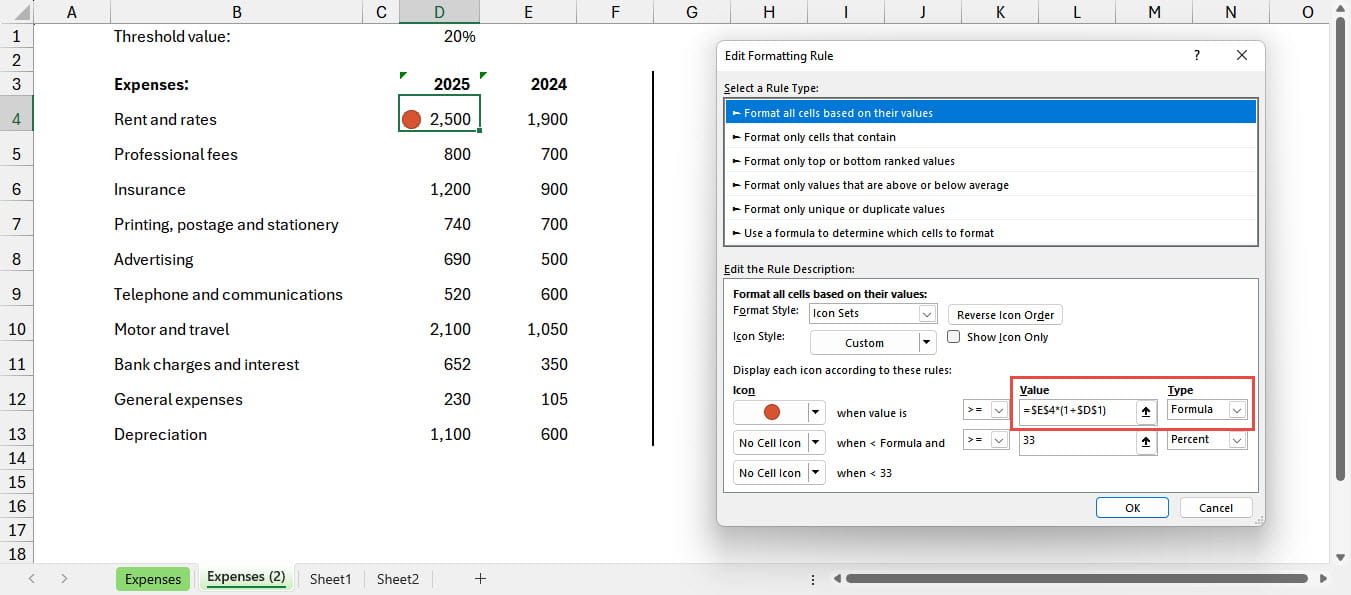
Rather than highlight the expenses items worthy of further investigation based just on their absolute value, it might be more useful to highlight those values that have increased by the highest percentage compared to the previous year. We can adapt our value in cell D1 to hold the threshold percentage and then work out a formula which will apply our conditional formatting icon based on this value. Here, we have just applied conditional formatting to a single cell, D4. We have set the rule type for our first icon to a Formula and calculated our trigger value as the value for the previous year, held in cell E4, multiplied by 1 plus our threshold percentage value:

=$E$4*(1+$D$1)

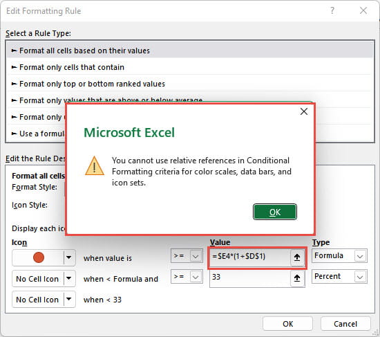
So far, so good. However, for this to be useful, we would want to apply it to all of the expense value cells in column D. We could try and do this by selecting those cells and changing our cell reference for the comparative year value to be relative:

=$E4*(1+$D$1)

However, when we attempt to accept our rule changes, we find that we can’t use relative values for formulas in the graphical types of conditional formatting rules:

Of course, we could set the conditional format for each of our cells individually, but this would be much more time consuming, and we would need to add the rule manually to any new rows that were added to our expenses list.

Show Icon Only

One solution is to use an additional column adjacent to the values that we want to highlight. In this column, we enter a formula that calculates our variance with just a simple formula that uses relative cell references:

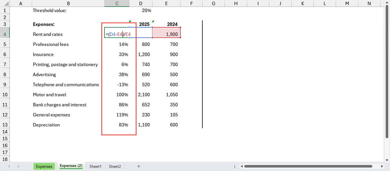
We can now add our conditional formatting rule to the variance values in this column:

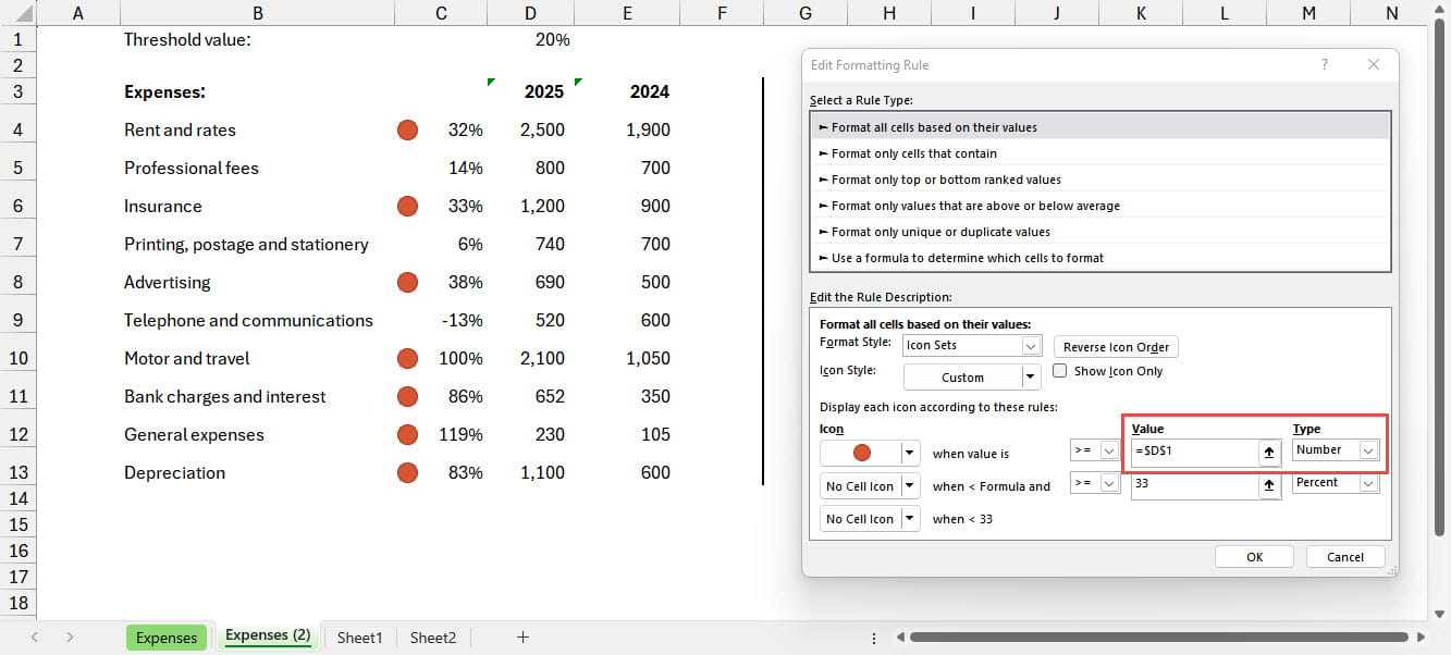
Although this successfully adds our traffic light highlight for those rows where our variance exceeds the threshold that we have set, it is quite a long way from the simple highlight that we were trying to achieve. In order to get rid of the unwanted distraction of the variance values themselves, we can use another of the detailed rule options: Show Icon Only. This will remove the normal cell contents and just display our conditional formatting icon. In the example below, we have turned on this option, reduced the width of column C, and aligned the contents of the cells in the column to be centred both vertically and horizontally. We have also changed the threshold value to 40% to demonstrate the calculation in operation:

Conclusion

Including a dedicated column for our highlight icons and using the Show Icon Only option allows us to apply a simple highlight based on a more complicated calculation.

In the next post in the series, we will have a look at the detailed rule options that are available when working with the other graphical conditional formatting rules: Colour Scales and Data Bars.

Additional resources

You can explore all aspects of Excel, including all aspects of the use of conditional formatting using the ICAEW Excel archive portal:

The 'Open in full-screen mode' icon in the bottom right-hand corner of the embedded report should show the contents at a more readable size with the Escape key returning you to the post.