Excel, what’s occurrin’ 7 – Conditional formatting from bottom to top

Introduction

The series so far:

• Excel, what’s occurrin’ – It doesn’t add up
• Excel, what’s occurrin’ 2 – Precision as displayed
• Excel, what’s occurrin’ 3 – Incomplete ranges
• Excel, what’s occurrin’ 4 – Number or text?
• Excel, what’s occurrin’ 5 – Getting iffy with it
• Excel, what’s occurrin’ 6 – Towards Zero

Conditional formatting

Conditional formatting applies any of a range of cell formats to cells depending on the values in those cells, or in other cells. Multiple conditional formats can be applied to the same cell or range of cells. If the formats are not mutually exclusive, they can all be applied when the condition is met. For example, one format can apply a cell font colour, another can apply a cell fill colour and a third could apply a cell border. Because all of these formats can be applied to the same cell or range of cells without affecting each other, all will be applied when the condition is met, regardless of the order in which the formats are set up.

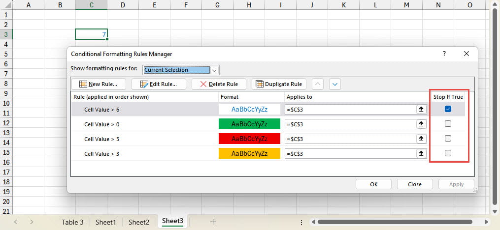
However, if two or more conditional formats all apply different cell fill colours for instance, then the order in which the formats are set up will be crucial in determining which of the formats is applied. In this example all of our conditions are met, and our three formats change the cell colour to green, orange and red. The question is. Which of the three formats will prevail?

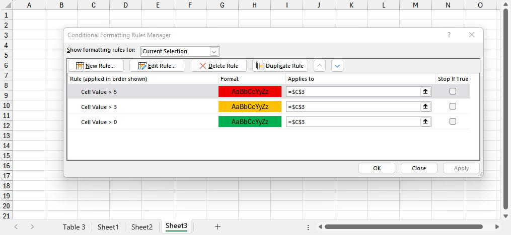
Note that, for simplicity, we have included our comparison values of 0, 3 and 5 directly in our conditional format rule. In real life, it would be better practice to include the values in cells and then refer to the cells, in order to make the way that the formatting works easier for users to understand and change.

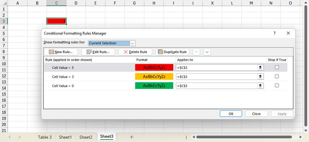
You might think that the Conditional Formats will be applied from top to bottom, so that the bottom format, the green cell fill, will be the one that will be applied, overriding the orange and red formats above it. In fact, the opposite is true. The order of the conditional formats actually represents the priority of the formats. Where multiple conditions are met, the one closest to the top of the list will be applied, as we can see here:

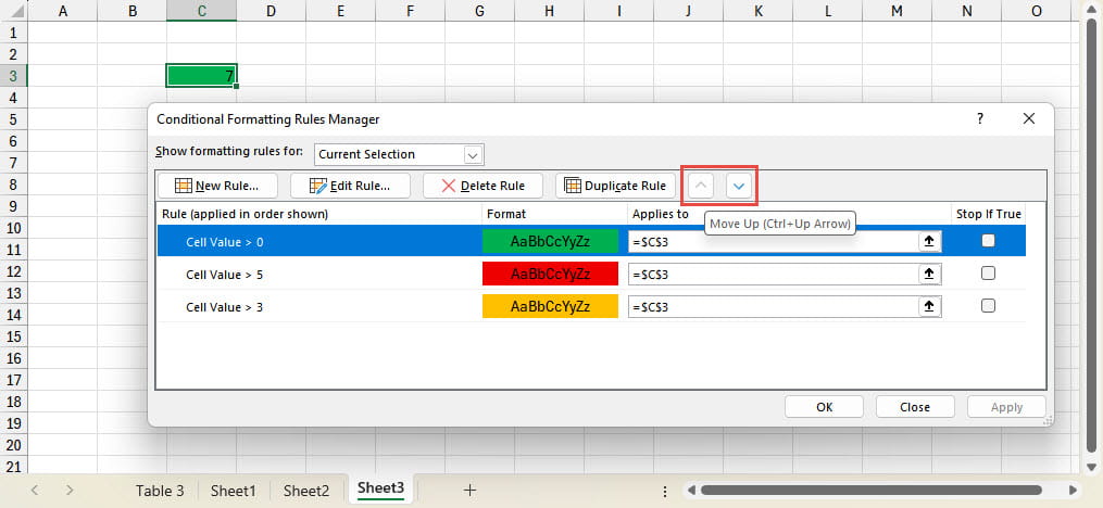
The Conditional Formatting Rules Dialog includes up and down buttons to change the position of our selected rule. If we select our green fill format and use the up button to move it to the top of the list, we can see that it now has a higher priority than the orange and red formats and is therefore applied to our cell:

Changing the order of rules is not the only way to control which rule is applied. There is also a Stop If True check box. This is only active for certain types of rule. The rules in the ‘Format all cells based on their values’ category cannot be set to Stop If True. Just to make things even more confusing, the Stop If True check applies from top to bottom. Here, we can see that our rule to change the font colour to blue is applied as well as our green fill colour:

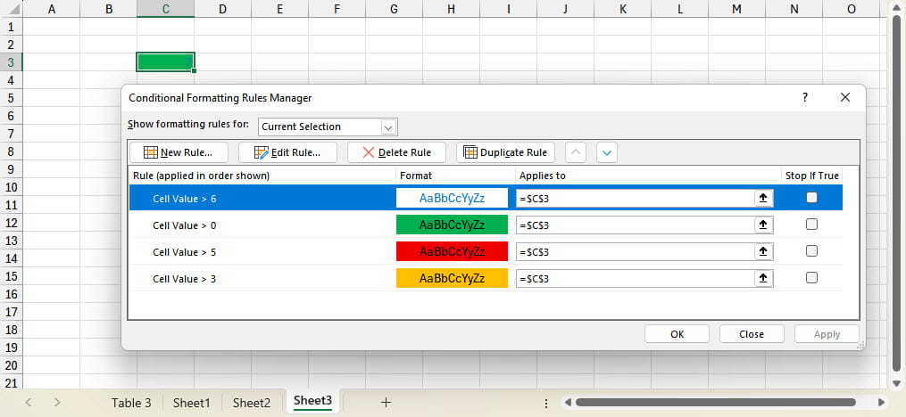
However, if we tick the Stop If True check box for our font colour rule, when the condition is true the rules below the rule will not be applied:

Conditional non-format

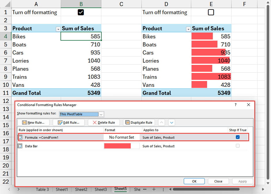
One possible use of the Stop If True option would be to allow a simple check box to be used to turn formatting on and off. In this example, we have applied red data bars to the Sales values within our PivotTable. We have then added a conditional format with no format that uses a formula to refer to the True/False value of a named cell into which we have inserted a Check Box using the Insert Ribbon tab, Controls group, Check Box command. Insert, Check Box is a relatively recent Excel introduction so might not be available if you are using an earlier version of Excel. We have placed the new rule above our Data Bar rule and turned on Stop If True:

Incidentally, there is a slight issue with this approach. If you set the Data Bar rule to Show Bar Only, once the rule is applied, suppressing the formatting will not restore the display of the values themselves:

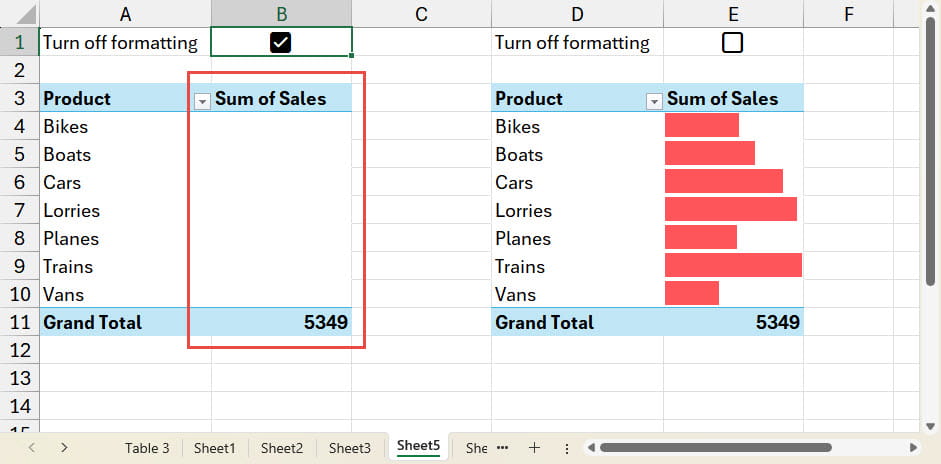
Refreshing the PivotTable will restore the display.

Next time

Next time we will look at Data Validation and see whether we’re all reading from the same sheet.

Additional resources

You can explore all aspects of Excel, including several articles on conditional formatting, in the ICAEW archive.