Excel, what’s occurrin’ 8 – Data Validation

Introduction

The series so far:

• Excel, what’s occurrin’ – It doesn’t add up
• Excel, what’s occurrin’ 2 – Precision as displayed
• Excel, what’s occurrin’ 3 – Incomplete ranges
• Excel, what’s occurrin’ 4 – Number or text?
• Excel, what’s occurrin’ 5 – Getting iffy with it
• Excel, what’s occurrin’ 6 – Towards Zero
• Excel, what’s occurrin’ 7 – Conditional formatting from bottom to top

Data Validation

The primary purpose of Excel’s Data Validation feature is to ensure that users enter appropriate data into cells. For example, if dependent Excel formulas expect a cell to contain a month number, Data Validation can be applied to the cell to prevent a user entering a month name or month number 14, 0 or -1 for example:

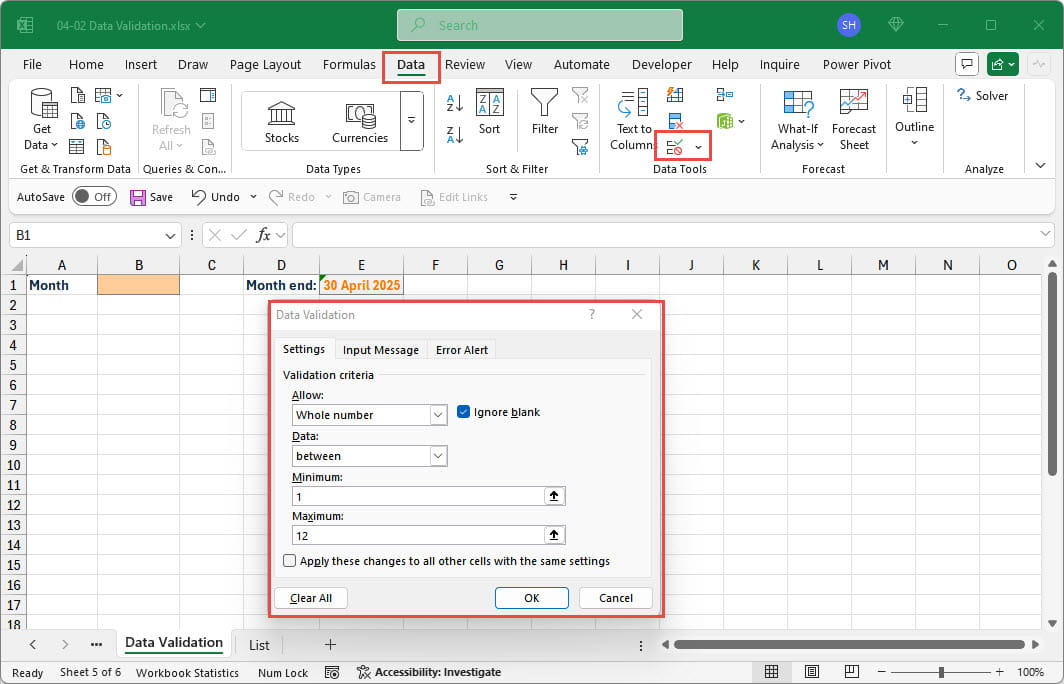
As we can see, as well as choosing to allow whole numbers, as opposed to dates, times or text for example, we can set the range of whole numbers that will be accepted. We can also create our own Input Message that the user will see when they click on the cell to which Data Validation has been applied, and the Error Alert which the user will see if they enter a value that contravenes the criteria set. Details of the basics of Data Validation can be found in part 1 of a series on Data Validation in the Excel Community. Here, we are going to concentrate on a particular aspect of Data Validation: using a list as the validation source.

Using Lists

The Data Validation source can be set to be a list. This can be a list of items separated by commas, but is more usually a reference to a range of cells. Using a list not only allows the cell entries to be restricted to the specific items included in the list, but can also be used to speed up data entry by allowing users to choose a value from the list, rather than having to type it in in full. A recent update to Data Validation made this a lot easier by automatically excluding duplicate values from a list and automatically filtering the list to match any characters typed into the Data Validation cell. Perhaps even more significantly, the highlighted item in the list can be entered into the cell just by pressing the Enter key, meaning there is no need to switch between keyboard and mouse/trackpad:

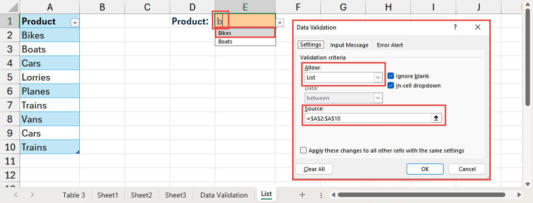
Having type in the letter ‘b’, our list is filtered to show the items that begin with b, with Bikes highlighted at the top of the list. Pressing the return key will enter Bikes into our validation cell.

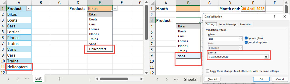
Useful as the use of lists in Data Validation can be, it does come with its own Excel oddity. If the range of cells used as the source of the list is a column table, the list will automatically include items added to the Table column – but only if the Data Validation cell and the Table are on the same sheet. In the following example, we can see that when we add ‘Helicopters’ to our Table, the Data Validation dropdown list on the same sheet automatically includes the new item, whereas the Data Validation cell on a different sheet does not:

In fact, going back through the history of Excel, when Data Validation was first introduced, it wasn’t even possible to refer to a range on a different sheet as the List source.

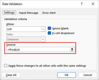
Before the advent of Dynamic Arrays, the easiest way around this limitation was to allocate an Excel Range Name to the Table column. The name could then be used as the source for the Data Validation list. Whichever sheet the Table is on, the range referred to by the Range Name will expand as the Table column expands thus ensuring that the Data Validation list will expand to include any items added wherever in the workbook the Data Validation cell is located:

Dynamic Arrays now provide an alternative. We can use a Dynamic Array formula to refer to our Table column and then refer to the cell containing the formula as our Data Validation source list, but using the # operator as a suffix:

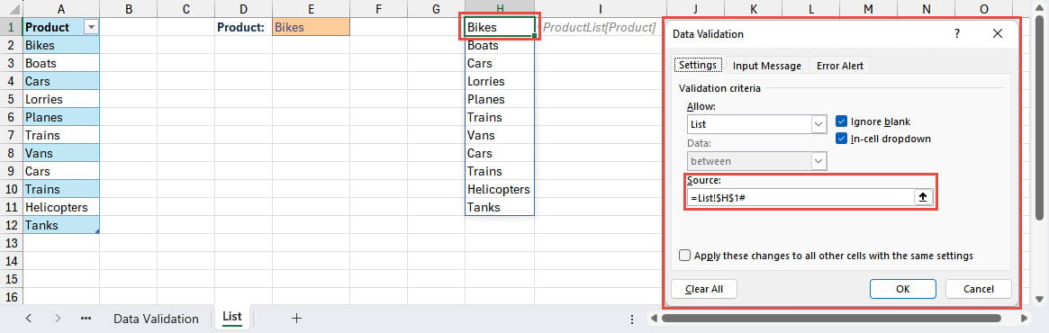
The # causes the reference to return the entire array that the Dynamic Array formula creates, rather than just the individual cell. Using a Dynamic Array formula also allows the use of one of the Dynamic Array functions such as SORT() or FILTER() to manipulate the list for presentation in the Data Validation list. You might think that the UNIQUE() function would be particularly useful in excluding duplicate items from the Data Validation list. However, the introduction of AutoComplete in Data Validation also automatically removed duplicate items from a list without the need to use UNIQUE().

Ignore blank

Just while we’re on the subject of Data Validation, you might have noticed the ‘Ignore blank’ check box. It’s quite difficult to work out what this is supposed to do. Amongst the things it doesn’t do is to remove blanks from a list that contains blank cells. It appears that it just applies when a user has entered a value outside of the Data Validation rules, and the Error Alert dialog displays an option to Retry entering the value. If ‘Ignore blank’ is turned on, the user can delete the entry in the Retry box and continue, and the entry will be accepted. If it is turned off, the entry will still be rejected. However, it does not prevent the entry just being cleared using keyboard Delete. outside of the Data Validation process.

Next time

Next time we will look at an automatic method of choosing items from a list and how easily it can go horribly wrong: why VLOOKUP() is now an ex-lookup.

Additional resources

You can explore all aspects of Excel, including several articles on Data Validation, in the ICAEW archive.