Excel, what’s occurrin’ 10 – a date with PivotTable destiny

Introduction

The series so far:

• Excel, what’s occurrin’ – it doesn’t add up
• Excel, what’s occurrin’ 2 – Precision as displayed
• Excel, what’s occurrin’ 3 – incomplete ranges
• Excel, what’s occurrin’ 4 – number or text?
• Excel, what’s occurrin’ 5 – getting iffy with it
• Excel, what’s occurrin’ 6 – Towards Zero
• Excel, what’s occurrin’ 7 – Conditional formatting from bottom to top
• Excel, what’s occurrin’ 8 – Data Validation
• Excel, what’s occurrin’ 9 – The wrong trousers

Aren’t PivotTables so last year?

Since the introduction of array formulas and, in particular, the GROUPBY() and PIVOTBY() array functions, some experienced commentators have suggested that the day of the PivotTable might be over. It is indeed true that the new formulas and functions can replace some uses of PivotTables. However, for many users, the complication of using formulas and functions, compared to the far greater simplicity of the PivotTable point and click approach, will be too high a price to pay just to avoid the need to deal with a manual or time-based refresh operation. In addition, it is currently much easier to format PivotTables, including using conditional formatting, and also to build in interactivity. Of course, dynamic array formulas will continue to improve and might well become a more practical way of replacing more uses of PivotTables in the future.

If you would like to explore dynamic array formulas and functions as an alternative to PivotTables, a recent Excel webinar provides an excellent example of what is achievable and how much additional complexity is involved:

• Is this the end of Pivot Tables? 

My dates aren’t working out

Having attempted to justify the continued relevance of PivotTables, we are going to examine a specific problem that you might come across when dealing with columns containing dates in the PivotTable’s data source.

Here we have a couple of thousands of rows of data and we want to see how the performance of our sales team compares year by year. We click anywhere in our Table of data and choose Insert Ribbon tab, Tables group, PivotTable. We would normally put our PivotTable on its own worksheet but, for demonstration purposes, we will position it next to our source data. All we need to do then is to click on the Sales field and the Salesperson field checkboxes in our PivotTable Fields pane. We’ll then drag the OrderDate field to the Columns area:

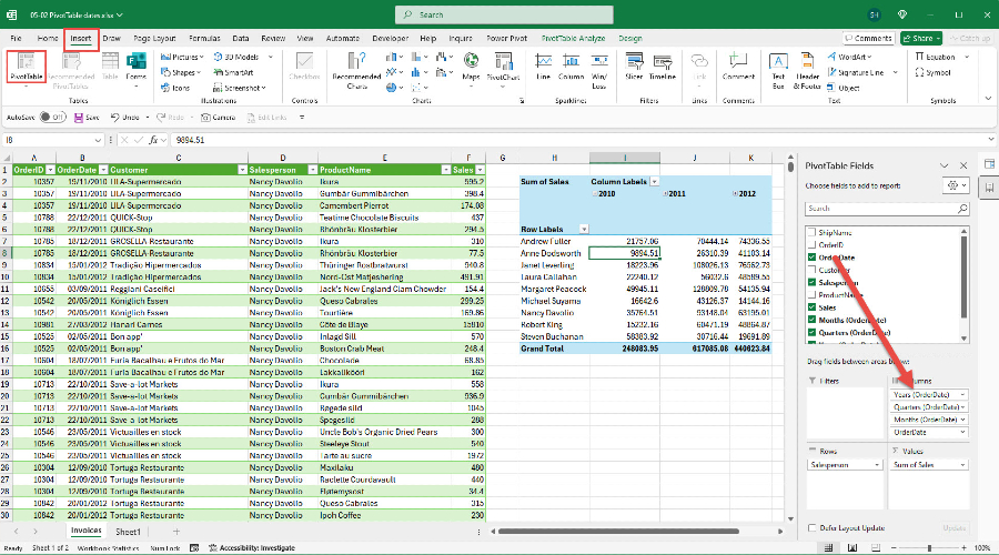
In less time than it takes to type in =GROUPBY, we’ve created our PivotTable and grouped our order dates by year.

Let’s try this again with a slightly edited set of data:

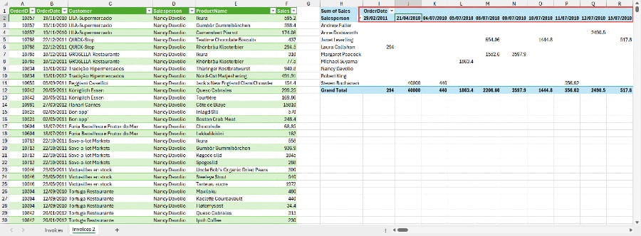
This time, we can see that our dates have not been grouped, but a column has been added for each unique item in the OrderDate field.

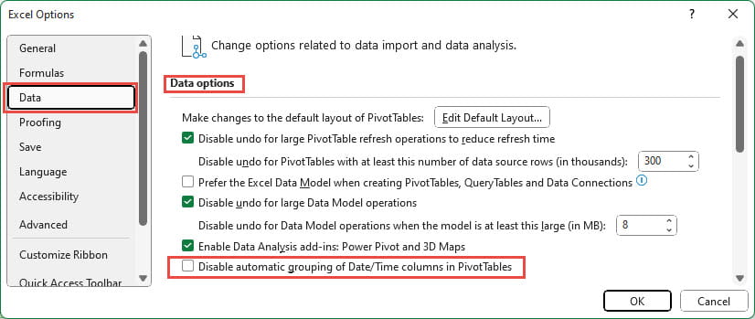
There are a few things that can cause this. In versions of Excel before grouping dates in PivotTables became the default, dates will be presented as individual values. In more recent versions, there is a specific option in Excel Options, Data category, Data options section to disable automatic grouping:

In both these situations, it is possible to right-click on any individual date heading and choose the Group… option to choose the date groupings that you would like to apply:

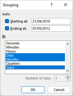
Note that, should you wish to group by week, you can choose Days to group ‘By’ and then set the ‘Number of days:’ value to 7. The ‘Starting at:’ date can then be used choose which day of the week you want your week groups to start on.

However, regardless of the version of Excel that you are using, you might find that, when you choose Group… from the right-click menu, rather than seeing the Grouping dialog, you see a message saying:

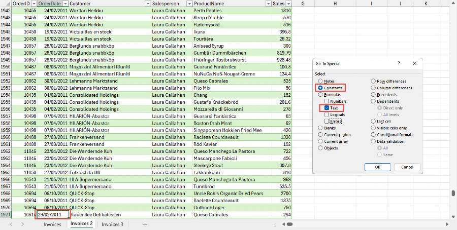
Cannot group that selection

This happens if your column of dates contains a value that Excel does not recognise as a valid date – such as 29/02/2011. In this case the solution is to make sure that your source data only contains valid dates. One way to identify where your invalid date, or dates, lurk is to use the Goto, Special dialog (keyboard shortcut F5, Special button) to search the entire date column for text values:

By the way

Not that it’s got much to do with the date issue but, just to land another blow in the ‘not dead yet’ discussion, we’ve taken an extra 29 seconds to customise our original PivotTable. We’ve applied conditional formatting to our OrderDate field values (so that the formatting adjusts dynamically to the addition/removal of rows or columns), changed the number format of the totals and edited the headings:

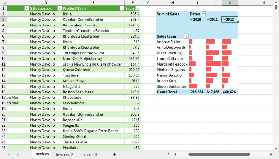
Take that, dynamic arrays.

Next time

Next time we will look at why it’s important to be aware of your Excel options.

Additional resources

You can explore all aspects of Excel, including many articles on PivotTables, Interactive Dashboards and dynamic array formulas and functions, in the ICAEW archive.