Partial Unpivoting

I have set myself some conditions:

• the formula needed to be in just one cell (no “helper” cells)
• no Power Query / Get & Transform or VBA: I want something that refreshes automatically
• the formula needed to be flexible, so that if we adjusted the number of rows and / or columns of the input table, the formula should still work
• obviously, the numbers of rows / columns of the output table could not exceed the row / column limitations of Excel.

You can find our Excel file here which demonstrates my solution. However, before explaining the calculation, allow me to clarify how I produced it first.

Brainstorming

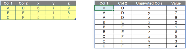
Firstly, inputs of the formula include:

• Data table (which is the yellow input table above)
• number of columns that will not be unpivoted, which is two [2] (i.e. Col 1 and Col 2). I will name this value as ColstoKeep.

Therefore, the number of columns to unpivot is three [3], which is calculated as below. We name this number as UCols.

=COLUMNS(Data[#All]) – ColstoKeep

Next, I need to consider some features (e.g. numbers of rows and columns) of the output array. After I unpivot the table, they should be calculated as below:

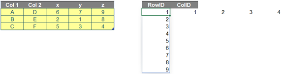
• Number of rows: 9

  =(ROWS(Data[#All]) - 1) * UCols

• Number of columns: 4. The output table will include the first two [2] columns of initial table and two [2] additional columns for the old Row Headers (i.e. x, y and z) and Values (i.e. numbers in Data table in this case).

  =ColstoKeep + 2

Then, I need to create a dynamic range for the output, so I will use INDEX and SEQUENCE. The row and column index numbers of output need to be created by SEQUENCE as follows. Let’s call them RowID and ColID.

• RowID:

  =SEQUENCE((ROWS(Data[#All]) - 1) * UCols)

• ColID:

  =SEQUENCE(1, ColstoKeep + 2)

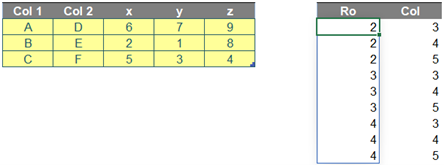
Additionally, I need to identify row and column positions of the Values in Data. Let’s call them Ro and Col. For example, number ‘7’ is located on row 2 and column 4 of Data.

• Ro:

  =ROUNDUP(RowID/UCols,0)+1

• Col:

  =MOD(RowID-1,UCols)+1+ColstoKeep

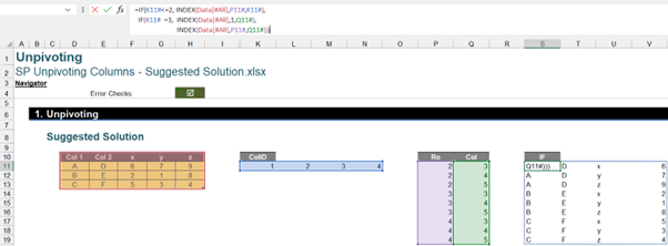
Finally, the trick here is to use ColID with an IF statement (below) as a connector for three [3] different INDEX functions, i.e.

“If ColID is less than or equal to ColstoKeep, then get the first two [2] columns of Data, else if ColID is equal to ColstoKeep + 1, then get the Row Header of unpivoted columns of Data, else get the Values of Data.”

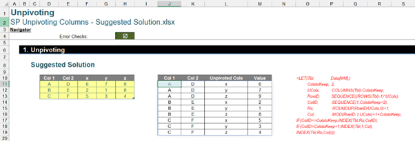
The result is as follows:

Putting it all together

If I want this all as one formula, I need to create a combination of all the described steps above within a LET formula (which defines names for the purpose of the formula only) as follows:

=LET(Tbl, Data[#All], ColstoKeep, 2,
UCols, COLUMNS(Tbl)-ColstoKeep,
RowID, SEQUENCE((ROWS(Tbl)-1)*UCols),
ColID, SEQUENCE(1,ColstoKeep+2),
Ro, ROUNDUP(RowID/UCols,0)+1,
Col, MOD(RowID-1,UCols)+1+ColstoKeep,
IF(ColID<=colstokeep,index(tbl,ro,colid), if(colid="colstokeep+1,index(tbl,1,col)," index(tbl,ro,col))))

There are seven [7] variables:

• Tbl is an input table to unpivot
• ColstoKeep is the number of first columns you do not want to unpivot
• UCols is the number of unpivoted columns
• RowID and ColID are row and column indices of the output table
• Ro and Col are initial row and column positions of Values in the input table.

Then, the final part of the formula is the calculation to unpivot the last three [3] columns, viz.

Although it is a long and complex formula, you can apply it to your input table by only replacing the values of Tbl and ColstoKeep. Perhaps this is just one of those formulae best to keep somewhere safe for when you need it…