Excel speed up productivity tricks – Data Set up

The previous blog in this series was on Formulas.

This article is about data set up. It doesn’t lead to productivity tips off the get go, but setting it up properly will speed you up when you later use the file.

Use Tables:

If you’re thinking “I already am – Excel is a table”, then you’re missing out on one Excel’s most important features. You’ve created Tables in Word or other apps by clicking Insert Tab > Table, well not many users know that Excel’s Insert tab has one too, if you select your data first, this has many speed benefits including.

1. Choose any style: Preset header colour, alternating colours etc.
2. Format on a table basis: Rather than cell by cell formatting, dragging formulas or pasting doesn’t mess up formats anymore.
3. Automatic growth: As you type to the right of the table or below it, formats, formulas, referencing will grow.
4. Amend the style by ticking/unticking the icons on the middle of the Table Design tab: Banded Rows, First Column etc.

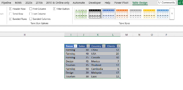
5. Get a total automatically by clicking “Total Row”: A dropdown in each to pick between sum, average, count etc. appears when you click in any cell.
6. When you type in a formula in a column, then press Enter, the formula automatically populates in the whole column.
7. The top table row is automatically using freeze panes, so if you scroll down when the table is in view and you’ve selected a cell in the table it shows the headers.
8. Simpler to understand formulas: Formulas refer to named columns rather than E5 or H6:H12, this applies to:

a. An entire column, =SUM(Data[Sales]) adds numbers in the column called “Sales”, in the table called “Data”, and includes new cells as rows are added below.

b. A cell in the same row =Data[@Sales] refers to the value in the Sales column in the current row.

9. Rename the Table: Brand new feature for Oct 2026 – when you create a Table, you can name the table there and then, otherwise you need to click in the Table > Table Design > Rename on the left.
10. You can convert your Table back to a range by clicking “Convert to Range” on the top left. There are other useful features there too.

11. Creating a Table has two shortcuts Ctrl T and Ctrl L, the latter being because the feature used to be called a List.

Simplifying printing in Excel

Printing in Excel is so unnecessarily complicated, there are dozens of options, and most spend way too many clicks to manually guess sizes. Who would want ever want one of 12 sheets to be printed to look like the screenshot here, follow these tips:

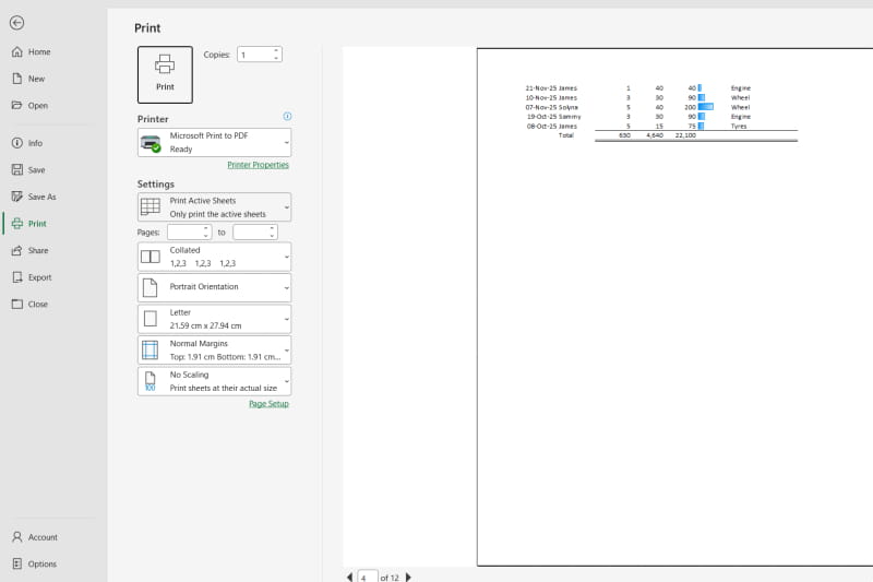
12. Landscape 1x1: Computer screens are horizontal so the default should just be “Landscape” and Width 1 page x Height 1 page. This alone clears up around 80% of printing needs.

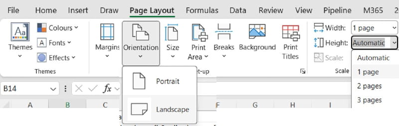
13. Print on multiple pages: If your data is too small, set it to print on multiple pages, by adjusting the “Height”, but then you also need to click “Print Titles” and select the table header row in the “Rows to repeat at top” option. This should cover around 15% of printing needs.
14. Print selection: Select the cells > File > Print > Print selection. These three steps should account for 99% of printing needs – the main exception is where you have multiple tables of different shapes in one worksheet.
15. Print multiple sheets or set printing options for multiple sheets in one go: Ctrl clicking the sheet tab names and then adjust settings. Note you can also make other changes to multiple sheets in one go like type in text, adjust formatting but I find it risky outside of printing as you could be overwriting en-masse without seeing what you are doing.

Data validation, cell protection & checkboxes

When creating a good data input form, you should prevent the wrong type of data going into a cell, databases are built on this, but Excel usually doesn’t do that meaning it takes a long time to clean once you set it up leading to errors. It prevents people writing “Female” in a column for gender that already has “Women” or typing “UK” in a country column which already has “Great Britain” etc. It also prevents typing in “Mon 14” in a date column or “Not sure” in a numerical column. A database would typically require a data type for each column, and so those using Excel to emulate databases this tool is essential. The video has the instructions or written out below.

16. Create a dropdown list: First create a list, sorted A to Z, then select the column > Data tab > Data validation > Choose List, and click the icon to select the list from elsewhere.
17. Set up number/date validation: Follow the instructions in the step above but instead of List, choose date, whole number or decimal and enter your minimum/maximum. Even if it can be any number it’s better to use 0 or -999999 as a minimum to avoid people entering wrong data inside it.
18. Insert checkboxes: Select one or more cells, Insert tab > Checkbox. You can then click to tick
19. Tick/untick checkboxes en-masse: Select several checkboxes and hit spacebar
20. Pasting data validation: Copy cells > Select destination > Paste Special > Data Validation
21. Circle invalid data: Validation is important to prevent future errors but can also be used to detect existing errors. Data tab > Data validation dropdown > Circle Invalid Data.
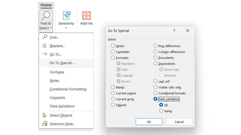
22. Using Go To Special to test data validation: Validation breaks far too easily sadly, especially by pasting in data into a validated cell. Select cells > Home Tab > Go To Special > Validation can show you all the cells which have validation. You get two choices:

a. “All” selects all cells regardless of what validation.

b. “Same” selects the cells with the exact same type of validation as the selected cell.

23. Locking spreadsheets the built-in way: This is a two-way process which I find counterintuitive and a bit limiting, so I prefer my own method mentioned later:

a. Before locking select the cells you want editable, right click > Format Cells > Protection tab > Unlocked

b. Click Review Tab > Protect Sheet, then tick the options you prefer and protect.

I personally find this limiting because most of the time users just want the cells to not be typed over but they don’t mind if the users builds charts, PivotTables, or uses Excel commands such as filters, grouping but many Excel options are greyed out after turning on standard spreadsheet protection, so I use an alternative method.

1. Locking all formula cells using data validation workaround:

a. Click Home tab > Find and Select > Go to special > Formulas > OK then every formula cell will be selected

b. Click Data tab > Data validation > select decimal > equal to > 67.726188 or any other number (which works like a password).

Copilot can help

Copilot is great at speeding data set up robust data in various ways, Edit with Copilot is available to all Microsoft 365 users with a premium license or those without a Premium license if they work in an organisation with under 2000 people. Click the Copilot icon on either the bottom right of the screen or the top right of the Home tab.

25. A three-word prompt “Clean this Data”: This can fix numbers stored as text, dates entered incorrectly, misspelled words, inconsistent text such as “F” or “Woman” in a column expecting “Female”. Being AI based though it might not get it right all the time though.

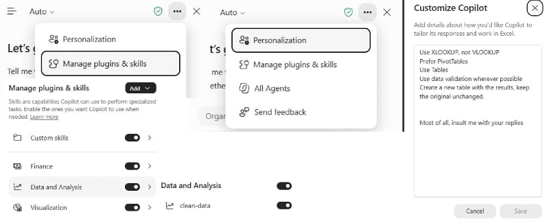
26. The new “clean-data” Skill: You can think of skills as prebuilt prompts or series of prompts, you must first enable the Skill by clicking the 3 dots on the Copilot pane > Manage plugins & skills > Data and Analysis > turn on clean-data. Then when you type your prompt, type @clean_data. Note that since this is brand new to October 2026 it is still being rolled out so may not show in your Excel or perhaps only in Excel Online.
27. The “brandkit” skill: Use @brandkit in Copilot to apply your brand to the current Excel file.
28. Create a custom skill: memorise and reuse a Copilot prompt for your specific use case, this may include a way to transform messy data which you regularly extract from a system etc. At the time of writing, create a Skill as described here but note that there will likely be a smoother process rolled out soon where you don’t need to leave Excel to do it.
29. Set up personalisation in Copilot: Specify what your copilot outputs should look like, such as “Use Tables always”, “format dates as dd-mmm-yy”, “make formula cells in pink”. Etc.

Below is a screenshot of how to enable built in skills and set up personalisation.

30. Workbook Rules: Personalisation works across your entire Excel whilst you can have a set of rules that works in the current file regardless of who opens it. On Copilot’s chat box click + Workbook Rules and specify.

That wraps up this fourth edition of speed up productivity tricks but check back in for another one in the coming months.