Excel Tip of the Week #372: Creating a depreciation schedule.

Excel has a small selection of functions for various ways of calculating depreciation built-in.

SLN

The “straight-line” function is the simplest:

=SLN(cost, salvage, life)

Cost is the cost of the asset

Salvage is the salvage value of the asset

Life is the number of periods over which the asset will be depreciated

SLN just replicates the formula:

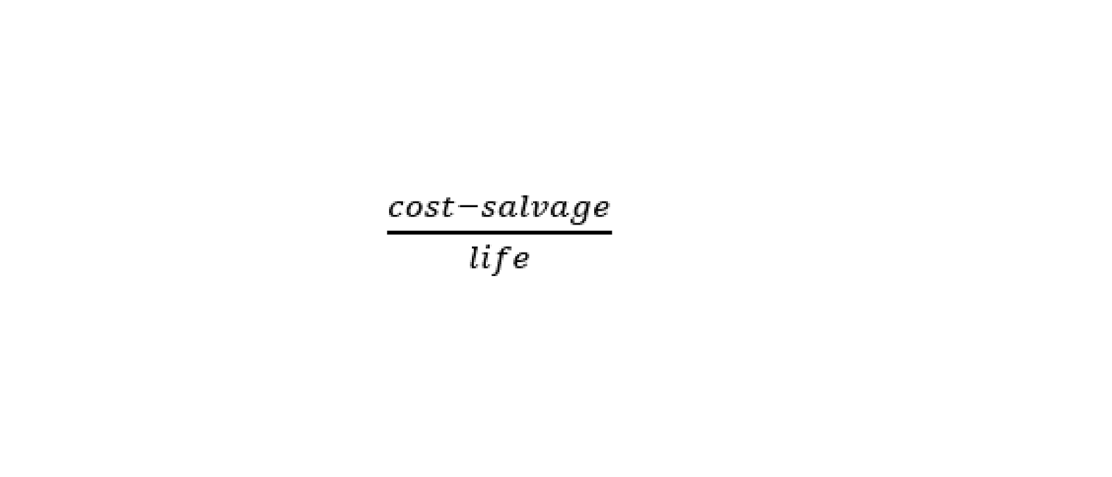
It’s arguably a little easier to read than typing the calculation directly, but ultimately nothing more. Notably, unlike the other depreciation functions, SLN has no input for which period is being calculated, and hence won’t automatically create the correct total amount of depreciation when copied along a timeline.

DB

This uses the declining-balance method.

=DB(cost, salvage, life, period)

Period is a number indicating which period the calculation is being calculated for

DB calculates depreciation such that the rate of depreciation applied to the net value of the asset is constant each month. The rate applied is rounded so the exact salvage value may not be reached after the full life of the asset.

DDB

This allows you to use the rare variant double declining balance method:

=DDB(cost, salvage, life, period, factor)

Factor is the rate that the depreciation is accelerated by – you can leave the number empty to use the default setting of 2.

This function is of very limited use.

VDB

This uses variable declining balance, which essentially is the same as double declining balance except it has the option to switch to the straight-line method once the depreciation from that would be greater:

  =VDB(cost, salvage, life, start period, end period, factor, no switch)

Start period is the period to calculate interest from

End period is the period to calculate interest to (these first two are usually set one period apart)

No switch can optionally be included if you want to switch back to the DDB method.

Once again, this function is of limited use.

SYD

This function uses the sum-of-years-digits method:

=SYD(cost, salvage, life, period)

This method front-loads depreciation according to the length of the asset’s life – so for example for a 12-period depreciation, the first period has 12 times the depreciation of the last one, the second has 11 times, and so on.

AMORLINC

Although designed for the French accounting system, this function can be useful as it can account for partial depreciation where an asset is acquired mid-period:

=AMORLINC(cost, date purchased, first period, salvage, period, rate)

Date purchased is the date that the asset was acquired

Rate is the depreciation rate applied each period (unlike all the other functions which compute this from a total useful life input)

Note that AMORLINC only works with year-long periods, and also requires both dates (the purchase date and the end date of the first period), as well as period numbers (which must start from 0 for AMORLINC). However, if you do all of this, then AMORLINC will automatically pro-rate depreciation in the first and last periods to end up with the correct total depreciated amount.

There is also AMORDEGRC, which applies a depreciation coefficient that scales with the useful life of the asset according to French accounting rules. You can see a demonstration of each of these functions and more in the attached workbook.

In most cases, none of the inbuilt Excel functions will work exactly the way we want. For example, while SLN can compute a monthly depreciation amount just fine, it doesn’t start or end automatically. The other functions above could do that, but are often difficult to interpret. So let’s set up a simple custom schedule instead.

The main thing we need to do is create something that will start and stop depreciation automatically. Here’s the basic layout, with all the manually-entered values we will be using:

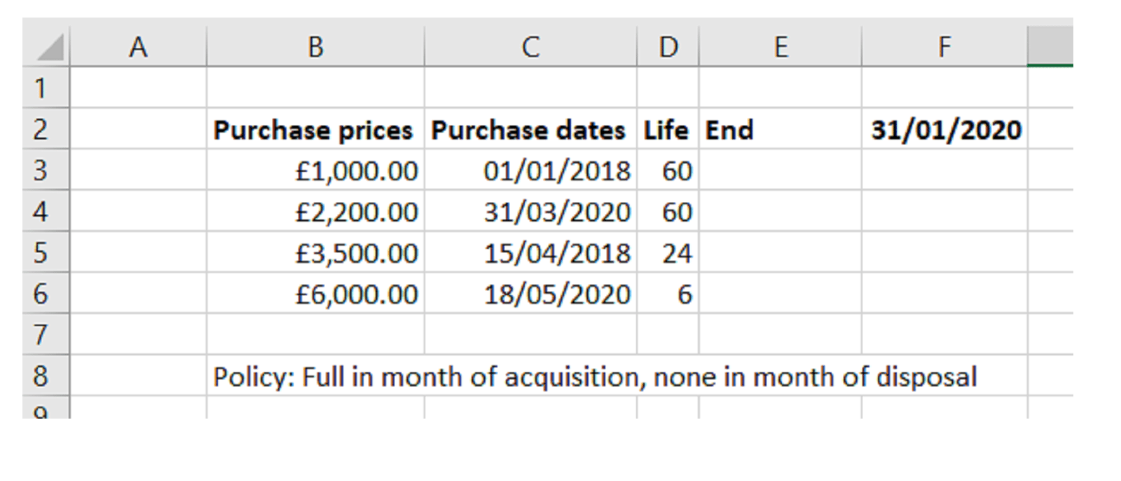
We can generate the rest of the month-end dates using:

=EOMONTH(previous date, 1)

And similarly fill in the period when the assets will become fully depreciated using:

=EOMONTH(purchase date, life)

Finally, for our schedule, we need to use an IF to make sure that 0 depreciation is calculated in the periods before the asset is purchased and after it becomes fully depreciated. The basic structure is:

=IF(AND(purchase date <= month-end date, end of depreciation date > month-end date), depreciation calculation, 0)

Note that we use less-than-or-equal-to for the acquisition calculation, to ensure a full month of depreciation even if the purchase is on the final day of the month, but a strict greater-than for the other check to ensure that none is charged in the final month.

You can see the completed schedule in the attached file.

If you have Office 365, then dynamic arrays are an option. We can make a version of the schedule that will automatically expand to include new items and will always show all required months.

We start up with this setup:

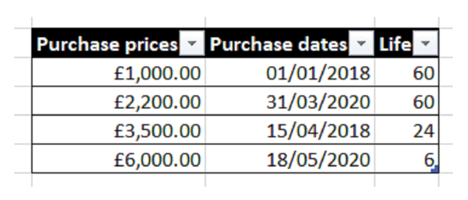
This is an Excel Table which I have named Input. Next we generate the list of the end dates using this function:

=EOMONTH(+Input[Purchase dates],+Input[Life])

The +s are a workaround due to EOMONTH being one of the functions that currently doesn’t play 100% nicely with dynamic arrays. But this will list our end periods, and will grow automatically as the data in the table is extended later on.

Now to make our headings:

=EOMONTH(MIN(Input[Purchase dates]), SEQUENCE(1, DATEDIF(MIN(Input[Purchase dates]), MAX(E3#), "m")+1, 0))

Breaking this down: We start with the earliest purchase date, and then create an array that outputs the month-end date moved on 0, 1, 2… months. The full length of the SEQUENCE function is determined by a DATEDIF which computes how many months there are between the earliest purchase date and the latest end date.

Finally, the dynamic version of our depreciation formula:

=IF((Input[Purchase dates]<=F2#)*(E3#>F2#), SLN(Input[Purchase prices], 0, Input[Life]), 0)

Note that we can’t use AND in an array – that would collapse the array into a single value. We multiply the two tests instead.

And once again, if you have O365, you can check out the end result in the attachment.

You may also like

• Previous post – Revisiting ROW(S) and COLUMN(S) functions
• TOTW index
• Next post – The Twelve Formulas of Christmas