Excel Tip of the Week #420 - STOCKHISTORY and exchange rates

This was briefly mentioned in TOTW #384 on data types, which it’s related to, so you might want to read that article first.

How does STOCKHISTORY work?

The STOCKHISTORY function is only available in Excel 365, and relies on the dynamic array spilling behaviour that entails – so you won’t be able to use this function in older versions. It can be used to return a table of prices for stocks or currency pairs over time.

Here’s the basic syntax:

=STOCKHISTORY(stock, start date, end date, interval, headers, properties 1, properties 2, …)

Stock is the ISO-format stock ticker for the stock you want to identify – e.g. MSFT or XNAS:MSFT – or the ISO currency codes for the two exchange rates – e.g. GBPUSD.

Start date is the date you want to start your table at (or just the date you want the value for if you are only returning one result).

End date is the end of the range of dates in the table

Interval is an option setting – 0 or blank for daily figures, 1 for weekly, or 2 for monthly

Headers is another option setting – 0 to excludes headers from your table, 1 or blank to include headers, and 2 to show both the instrument identifier and headers.

Properties is the final input to the function, and you can include several; this allows you to decide which columns are included in the table. The options are:

0 – The date of the data point
1 – The close price
2 – The open price
3 – The high price
4 – The low price
5 – The trade volume

You can include any number of these in whatever order you like; if excluded the default table includes the date and close price.

All this is fairly theoretical, so let’s look at an example, which returns weekly close prices for a given stock:

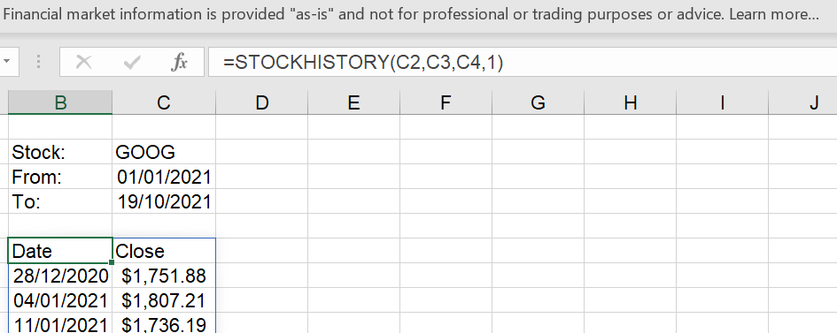
Note that this is a single function in one cell, which spills results into an array. Also note that any workbook containing one or more STOCKHISTORY functions will automatically also display a disclaimer from Microsoft each time it is opened, which you can see at the top here.

This function is very handy for making variable charts – but it does require a little set up. You can’t set a spilled dynamic array directly as the source of a chart, but you can set it as the definition of a named range, and then set the named range as the source. We also want to lose the headers for this one:

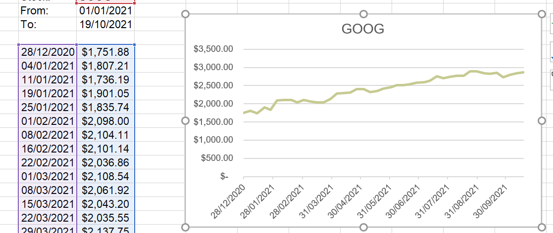
There are two defined names here:

StockChartSource: =INDEX('Stock tracker'!$B$6#,0,2)
StockChartLabels: =INDEX('Stock tracker'!$B$6#,0,1)

These are then set as the data and axis labels for the chart (you also have to specify which sheet the range names belong to). This way the chart will expand and contract as we amend the formula.

Making an exchange rate function with STOCKHISTORY

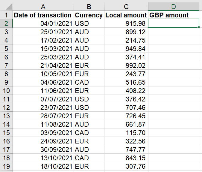
You can also use STOCKHISTORY to compute an exchange rate for use within a single-cell function. Let’s look at how we can build this up. We have the following:

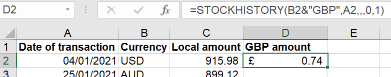
We can start with just a basic STOCKHISTORY function:

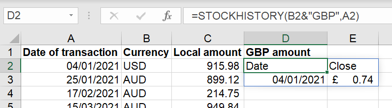
Note that we have used & to conjoin the currency code from column B with the text value “GBP”, as our home currency. As you can see, this shows us the rate for the given date in a 2x2 table.

We can then specify that we only want the close amount and no headers:

That gets us our rate – all that remains is to convert the local amount and round off:

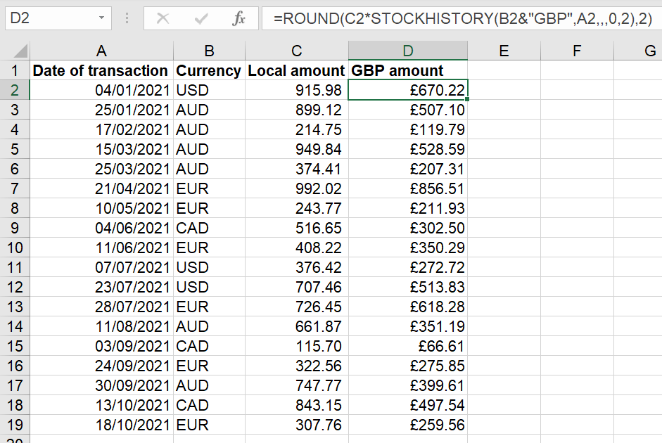
One note – using the close rate will actually lead to an error if the transaction date is today’s date. In the above we have used the open rate instead; alternatively you can either use an IF to pick the open rate if the date is today, or just leave the error – it will be fixed once the market closes and a close rate is available.

You can check out both of these examples in the attached file .

• Previous post - Revisiting macros and custom functions
• TOTW index
• Next time – Comparing lists redux!