Excel Tip of the Week #421 - Comparing lists redux

This was the subject of the very first Tip of the Week back in 2013, and was revisited in TOTW #120. We’re going to look at a few different ways of accomplishing the task.

Conditional formatting

The simplest method works for when you have two lists. Put the two side by side, select the whole lot, and use Home => Conditional Formatting => Highlight cells rules => Duplicate values. The result will be something like this:

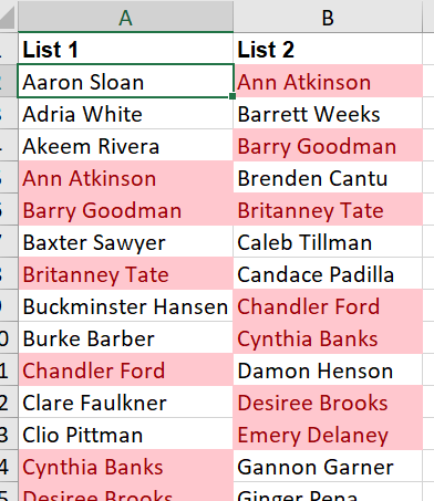
The overlap between the two lists is shown in red, and the items which are unique to each list are not highlighted. This makes comparison quick and easy.

With this method – and all the methods we’re looking at today – remember that Excel a) isn’t case sensitive, so Aaron, aaron, and AARON will all be treated as the same; and b) Excel isn’t psychic, so “Ann” and “Anne” will be treated as different, even if they’re supposed to be the same. This last point is particularly relevant for subtle things like accidental extra spaces – e.g. “Barrett” and “Barrett ” will be treated as different.

Formulas

This approach requires a “master list”, with each unique item listed once. You can make one by using Power Query (more on this later), or just by copying all the individual lists one on top of the other and then using Data => Remove duplicates.

The approach is then to use a formula such as COUNTIF to see if the item appears in a targeted list once, or zero times. You can use IF to reformat the answer into whatever text or calculation you want. Here’s the finished article:

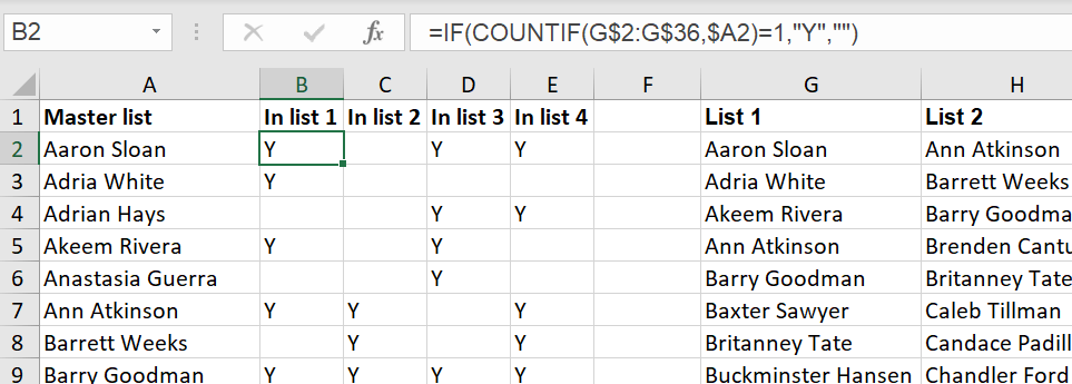
The formula here is:

=IF(COUNTIF(G$2:G$36,$A2)=1,"Y","")

Note that this has been written with $s to allow the same formula to be used in all four columns. Also note that it’s important to make sure that the range for the comparison is large enough – for example, list 1 only goes down to row 35, but some of the other lists reach row 36, so the formula needs to go to row 36 to avoid missing anybody.

Power Query

Finally, it is possible to make these kinds of comparisons using Power Query. While the setup is a bit more involved in that case, the advantage you gain is that the process is refreshable – you can add and change items in the individual lists as much as you like, and then regenerate the master list and all the comparisons with just a press of the Refresh button.

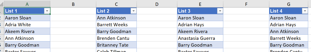
To start with, each of our lists needs to be stored in a Table:

We can then import these one at a time into Power Query with Data => From Table/Range. We are going to make a couple of quick tweaks to each:

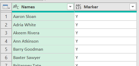
Firstly, we have renamed all the first columns for each query to a common heading, in this case “Names”. This will mean we can easily append them together in a minute. We have also added a custom column with a simple formula of =“Y” to display a Y next to every name. This will be what we pull through on the final comparison. After these quick changes, we then load each as a connection only.

The next step is to create our master list. To do this, we create a new query that appends all four of the individual lists:

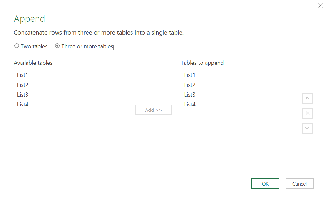
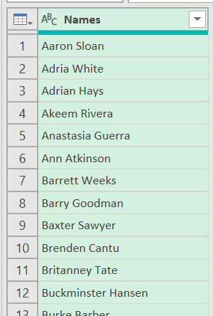
We can then remove the duplicates from the resulting one-column table and sort to get our master list. We will also remove the “marker” column from the result.

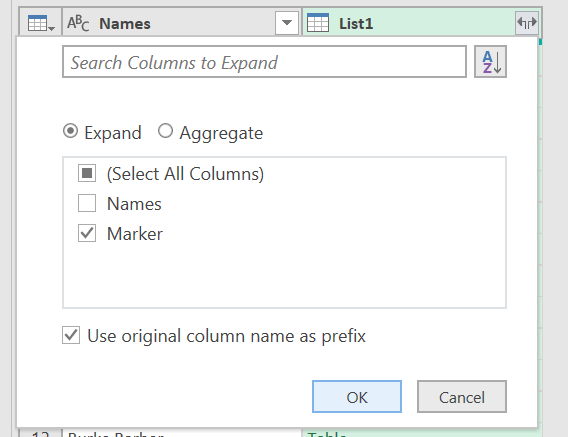
The next step will be to merge each of our individual lists, one at a time, and then expand the merge to show the “Marker” column only:

Do that four times, and then we can export the final result:

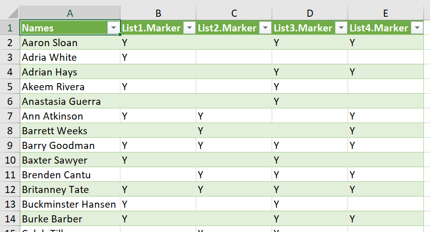
The comparison is complete, and we can refresh it easily when needed! You can check out this example, plus the other two, in this week’s example file.

Previous post - STOCKHISTORY and exchange rates
TOTW index 
Next time – Better error catching formulas!