Excel Tip of the Week #422 - Better error catching formulas

What’s wrong with IFERROR?

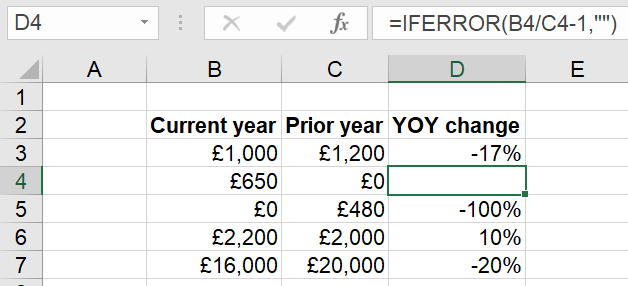
IFERROR is a helpful function that allows you to provide a backup value or formula to be used if the primary one returns an error. Take for example this year-on-year change calculation, which returns a blank if the prior year value is nil:

This works just fine; however the issue is that it over-catches. Any error of any kind will be hidden by this formula, not just dividing by zero. This means that the change formula is less useful for catching real errors. For example, let’s say that a current-year figure pulled through a non-numeric value:

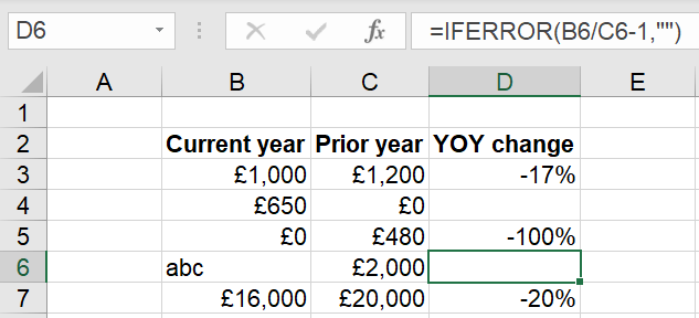
Now a reviewer is less likely to catch the mistake because the genuine error has been hidden by a formula that was only intended to tidy up divide-by-zero errors.

The best solution is to design your error-catching formulas only to catch a specific error. In this case, for example, you could use this instead:

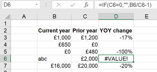
This formula only uses a blank for the specific issue of a zero denominator, and so the #VALUE! error is still shown for the row with a faulty input. Now the comparisons remain neat and tidy, but also still function as a way of spotting unrelated errors.

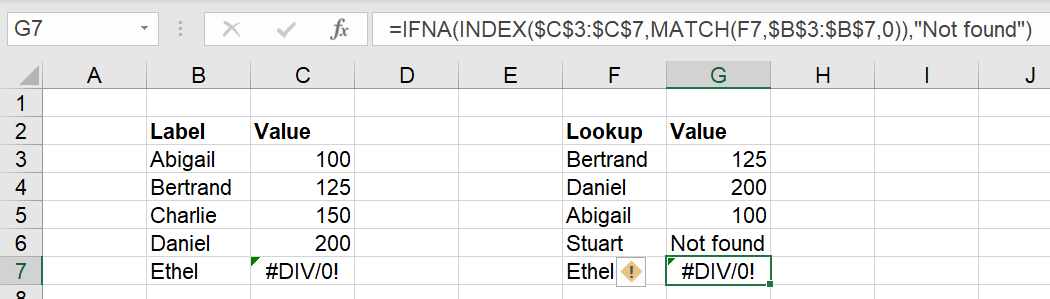
For one specific errors- the #N/A! error – there is an equivalent of IFERROR that only works for that one specific issue. The #N/A! error marks when a match can’t be found for a lookup function:

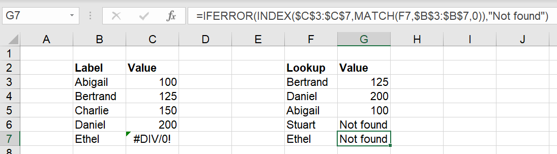
Here the IFERROR returns “Not found” for both the value for Stuart, which is not present in the lookup table, and for Ethel – which is present but contains a calculation error. A better alternative is to use IFNA instead:

Other kinds of errors

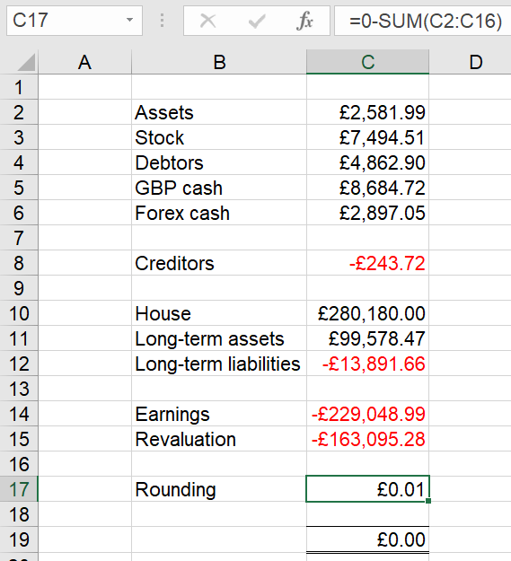
As well as literal Excel error values, error-correcting formulas also come in other forms. For example, here’s a naïve balancing figure formula used to correct small rounding errors from foreign currency conversions in a balance sheet:

All well and good so long as the problem is just some sub-decimal rounding, but this formula will “correct” any size of balance sheet issue – so if for example a fat thumb adds £70k to the stock figure by accident:

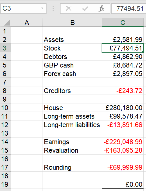
A careless reviewer could see the 0 balance and be tricked into thinking that things are OK, whereas of course something has gone very, very wrong. The better approach is to limit the rounding formula so that it can only operate on a fixed scale:

=IF(ABS(0-SUM(C2:C16))<0.01,0-SUM(C2:C16),0)

This allows the rounding formula only a penny tolerance, and otherwise returns 0 and lets the error come through.

There are plenty of other tricks like this – the key point is to think when you’re making any error catching or correcting formula, and make sure that you are only going to fix that one error, and not hide any other sins.

• Previous post - Comparing lists redux 
• TOTW index
• Next time – Our Excel Christmas list!