
Hello all and welcome back to the Excel Tip of the Week! This week, we have a Creator level post in which we’re taking an updated look at how to split one dataset into multiple ones based on a particular column, using formulas. This is an update of TOTW #196.
Traditional approaches
We’re going to use the same dataset as the original post for consistency:
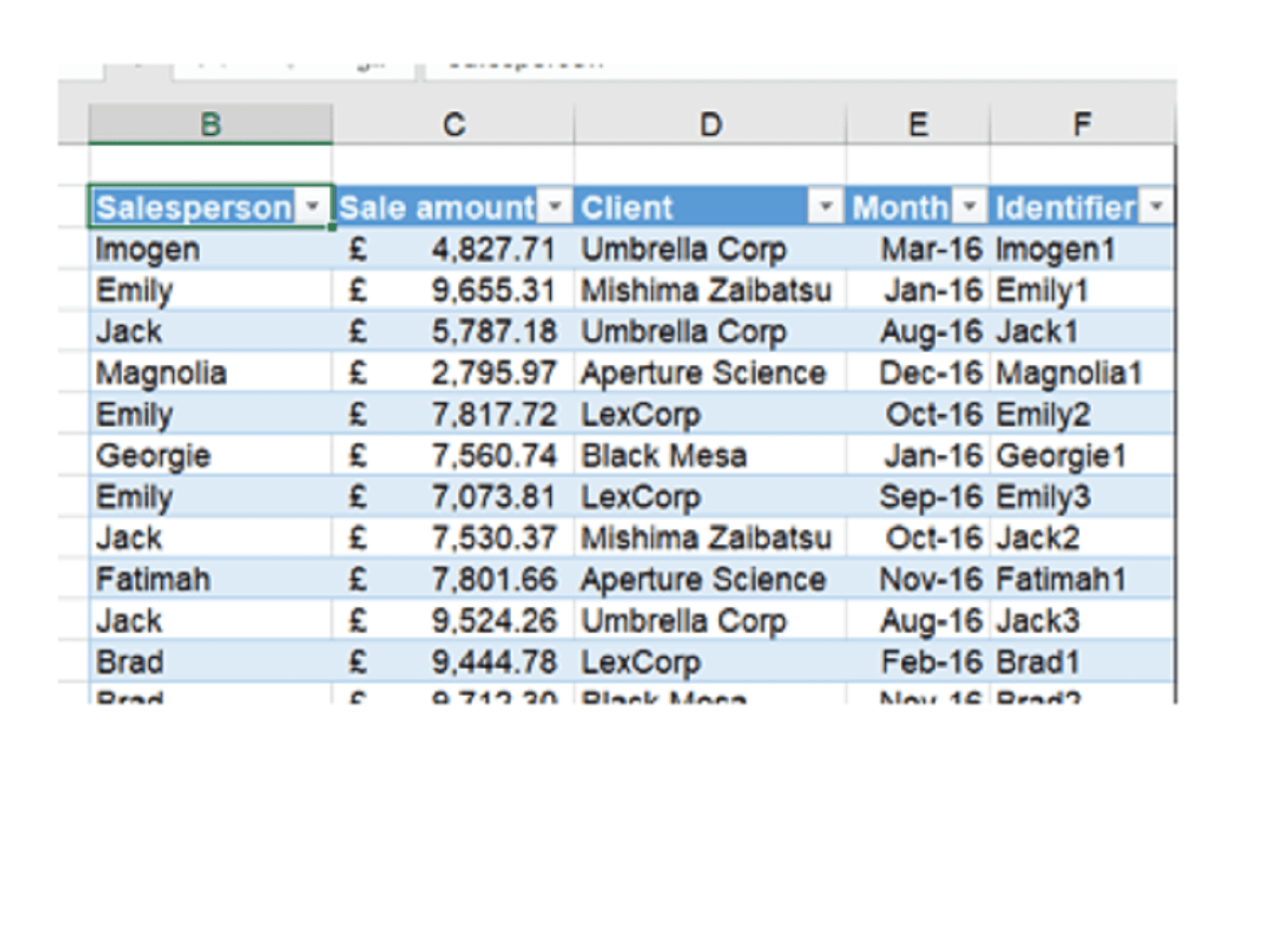
We have made this into an Excel Table because it will make referring to the data a little simpler later on (the Table is named Data). It also simplifies our “Identifier” column, which automatically identifies each row with the name of the salesperson and a number for which instance this is:
=[@Salesperson]&COUNTIF(INDEX([Salesperson],1):[@Salesperson],[@Salesperson])
The second part here looks at the number of times that salesperson’s name has appeared in earlier rows of the table. A similar effect can be achieved with traditional formulas and part-fixed references:
=B3&COUNTIF($B$3:B3,B3)
However this can go wonky when inserting rows; the Structured References version above is more consistent.
We want two different options: One to create a “pivoted” appearing list of all the data in just one field for each salesperson, and one to filter to get all the columns of data for a specific salesperson. For the first, we need to manually create a row of headers for each salesperson, then paste the following formula:
=IFNA(INDEX(Data[Sale amount],MATCH(H$2&ROW()-ROW(H$2),Data[Identifier],0)),"")
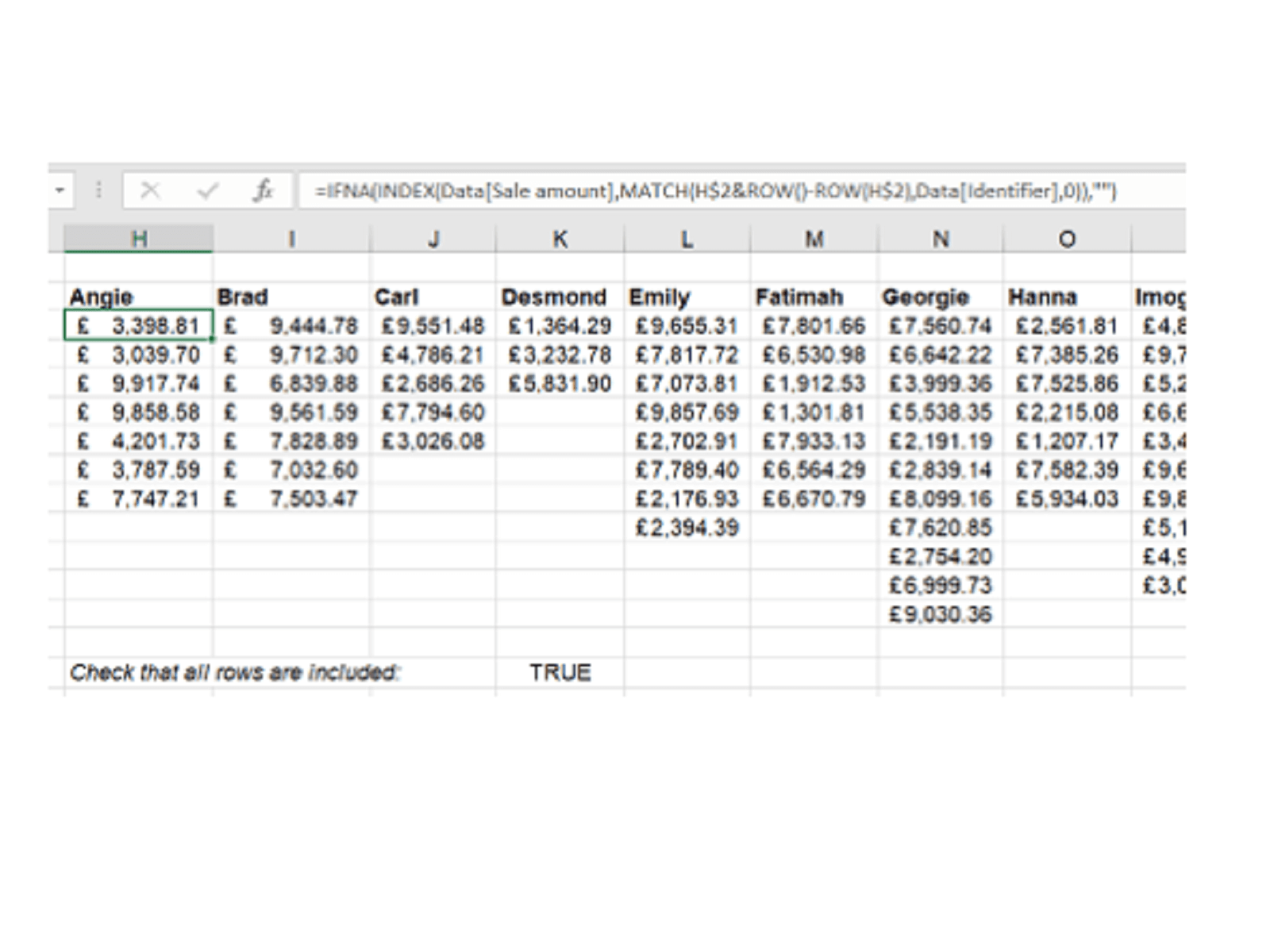
This formula uses the header value and the cell’s position in relation to it to figure out which identifier is needed, then uses an INDEX MATCH (see TOTW #201) to find it in the original Data table.
Because of the limitations of traditional formulas, the only way to make sure that all the original data has been brought across is to use a check formula:
=COUNTA(Data[Sale amount])=COUNTIF(H3:T13,">0")
A similar approach can be used for the filtering exercise:
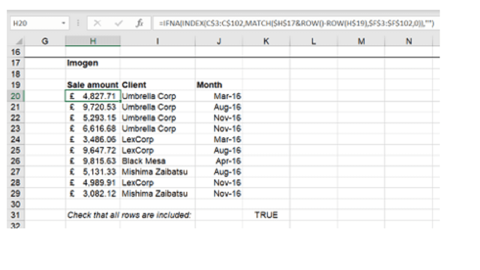
The formula here is:
=IFNA(INDEX(C$3:C$102,MATCH($H$17&ROW()-ROW(H$19),$F$3:$F$102,0)),"")
Note that here we are choosing not to use the structured formulas, instead using normal cell references with partial $s to allow the formula to be copied rightwards to grab each column in turn. And once again, we have to use a check to make sure that all the rows are included – because we will only pull through as many values as we have formulas pasted.
Dynamic arrays
If you are using Excel for Microsoft 365, then you have access to the new dynamic arrays calculation engine and its functions. While not perfect, these do offer some superior functionality when dealing with these kinds of tasks.
First of all, let’s look at the filtering task – one for which the perfect function exists:
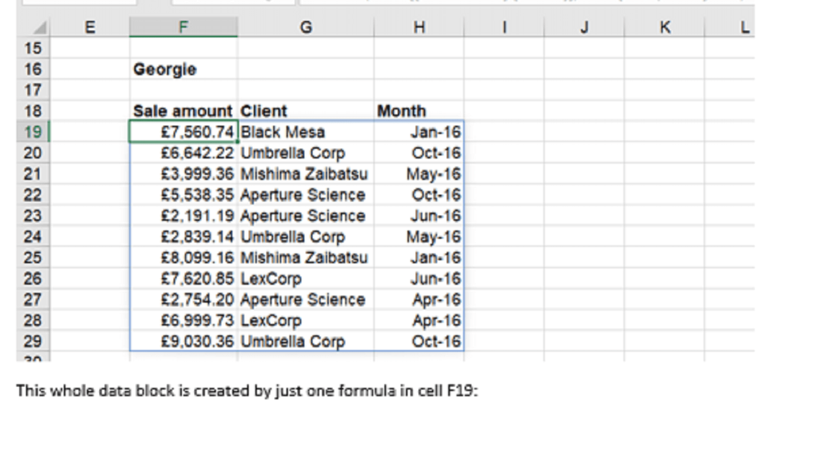
This whole data block is created by just one formula in cell F19:
=FILTER(Data2[[Sale amount]:[Month]],Data2[Salesperson]=F16)
This will automatically grow and shrink as needed to accommodate the data for the salesperson selected in the dropdown cell.
We can do something similar for the pivoted data:
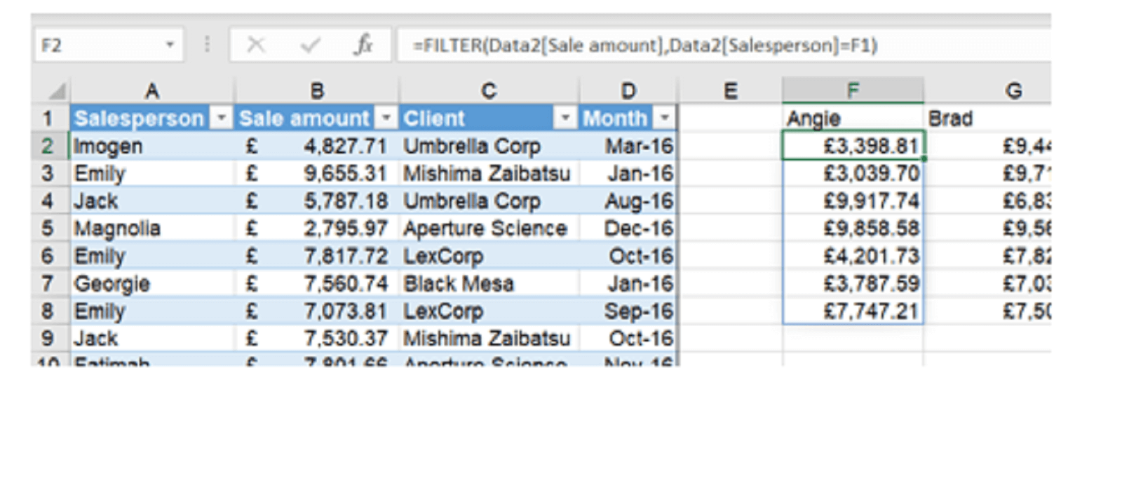
The formula being:
=FILTER(Data2[Sale amount],Data2[Salesperson]=F1)
We can copy this rightwards to make a list for each salesperson. But this isn’t perfect. We can get a list of the unique salespeople easily enough:
=TRANSPOSE(SORT(UNIQUE(Data2[Salesperson])))
But this doesn’t automatically copy our FILTER function rightwards if a new salesperson is added to the Table. You can check both examples in the attached file.
But there is one further step we can take that will handle the pivoted data case too – including adding new columns if new salespeople are added – by switching over to Google Sheets. Here we can use the powerful QUERY function to create an entire pivoted dataset with a single function:
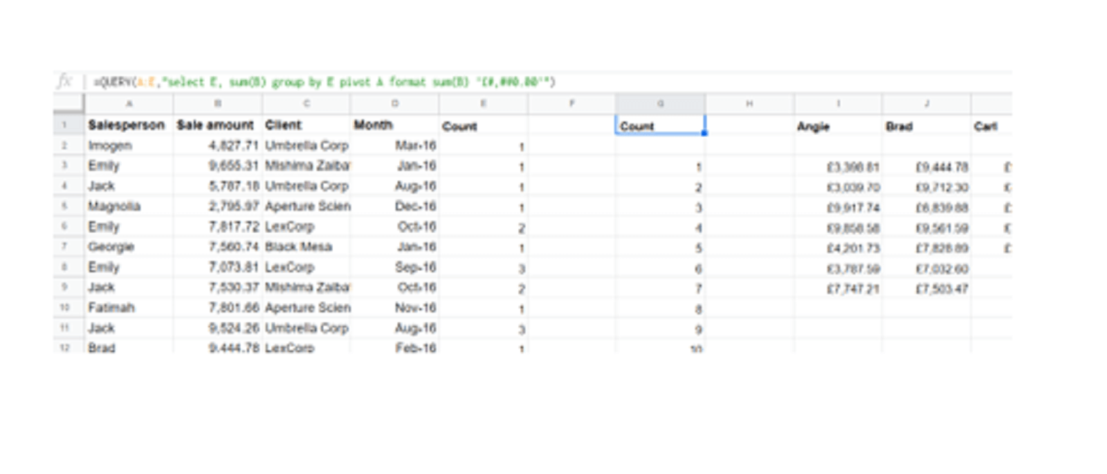
We have used a variation of the enumeration function from earlier in our data table:
=COUNTIF($A$2:A2,A2)
And this is the QUERY syntax for our pivot:
=QUERY(A:E,"select E, sum(B) group by E pivot A format sum(B) '£#,##0.00'")
This gets the entire pivoted data set from column G onwards – all with just one formula. Check it out here.
You may also like
Excel community
This article is brought to you by the Excel Community where you can find additional extended articles and webinar recordings on a variety of Excel related topics. In addition to live training events, Excel Community members have access to a full suite of online training modules from Excel with Business.

Archive and Knowledge Base
This archive of Excel Community content from the ION platform will allow you to read the content of the articles but the functionality on the pages is limited. The ION search box, tags and navigation buttons on the archived pages will not work. Pages will load more slowly than a live website. You may be able to follow links to other articles but if this does not work, please return to the archive search. You can also search our Knowledge Base for access to all articles, new and archived, organised by topic.
