
Hello and welcome back to Excel Tips and Tricks! This week we have a Creator level post in which we’re looking at new and improved ways of checking for and handling errors.
Error handling functions
There are a range of functions in excel that can check and handle errors in excel workbooks.ISERROR or IFERROR?
ISERROR can pick up all error types #VALUE!, #REF!, #DIV/0, #NAME?, #NULL! including #N/A errors.
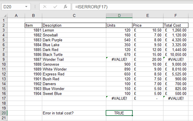
The function can be used to check for errors in the values and then return a TRUE value if an error is present:
=ISERROR(value)
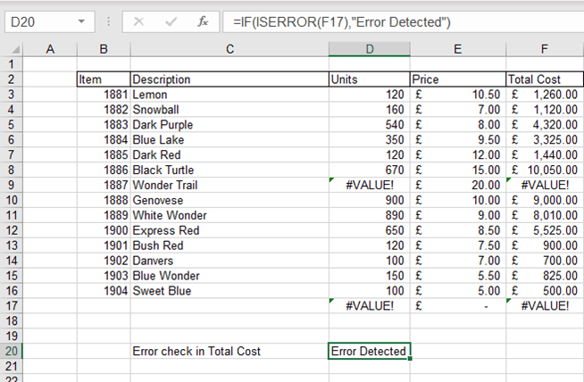
=IF(ISERROR(A1), “output”)
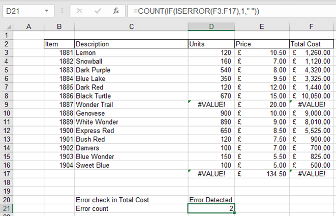
=COUNT(IF(ISERROR(CELL RANGE),1,” “))
Do note that IFERROR carries an inherent risk of ‘covering up’ errors if used inappropriately, so remember that it should only be used to flag errors, not make the errors go away.
Tips on how to use IFERROR (and how not to use it!) were covered in more detail in tip #422.
FILTER
The FILTER function in Excel is part of the relatively new set of array functions and is used to filter a range of data based on the criteria that you specify:FILTER(array, include, [if_empty])
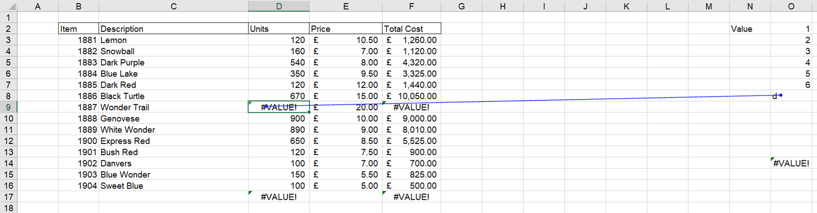
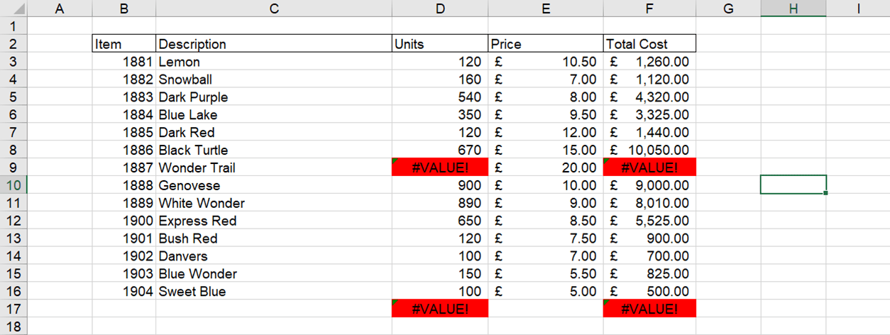
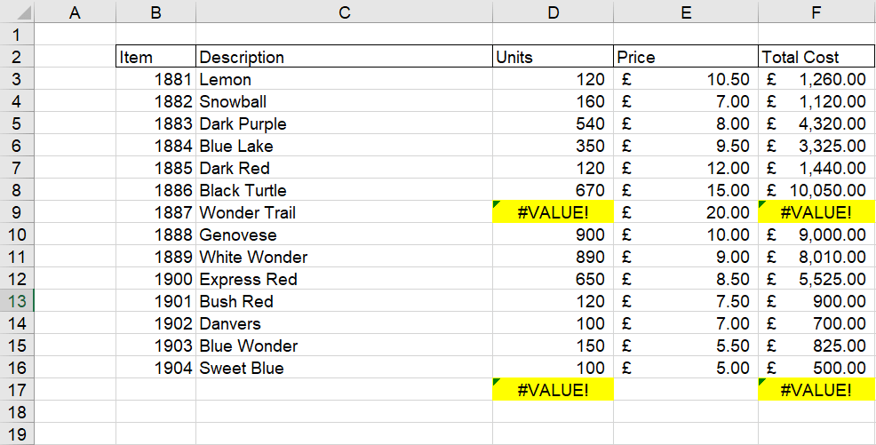
In the example data set below, I want to pull out information on items where there are errors in the total cost and units calculation.
To do this, the FILTER and ISERROR functions can be combined to filter the data where errors have occurred:
=FILTER(array, ISERROR(range))
The formula above provides me with the following output where I can clearly see the item number, description and then details of the error:

XLOOKUP
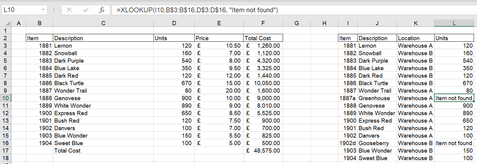
We introduced XLOOKUP in tip 337 as a more flexible and reliable alternative to VLOOKUP. As an added benefit, XLOOKUP has an option to handle #N/A errors.For example, in the data set below I would like to find the units of different items using XLOOKUP. However, if information regarding an item is missing, I can enter a value into the optional 4th argument to replace a #N/A error with the specified output:
=XLOOKUP(lookup_value, lookup_array, return_array, [if_not_found ])
Again, remember that this shouldn’t be used to cover up the error, rather to make it easier to manage. In the example below, by identifying where information is missing we can follow up on this error to resolve it.
Built-in Error Checking
Error checking
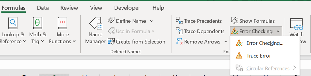
Another way to check for errors in formulas in excel is using the built-in ‘Error Checking’ in excel in the formula auditing tab.
The dropdown offers three options including:
- Error checking
- Trace error
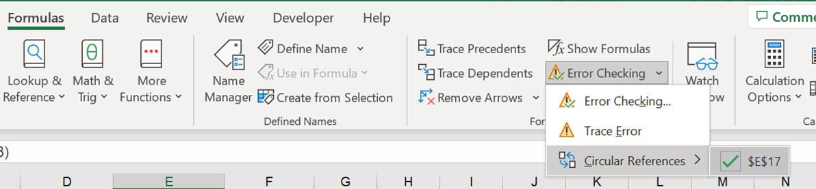
- Circular References
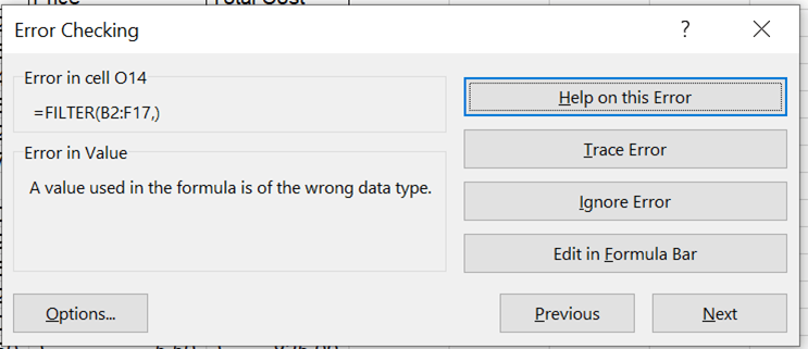
You can then use error checking to either trace the error, ignore it, or edit the formula.
Conditional formatting
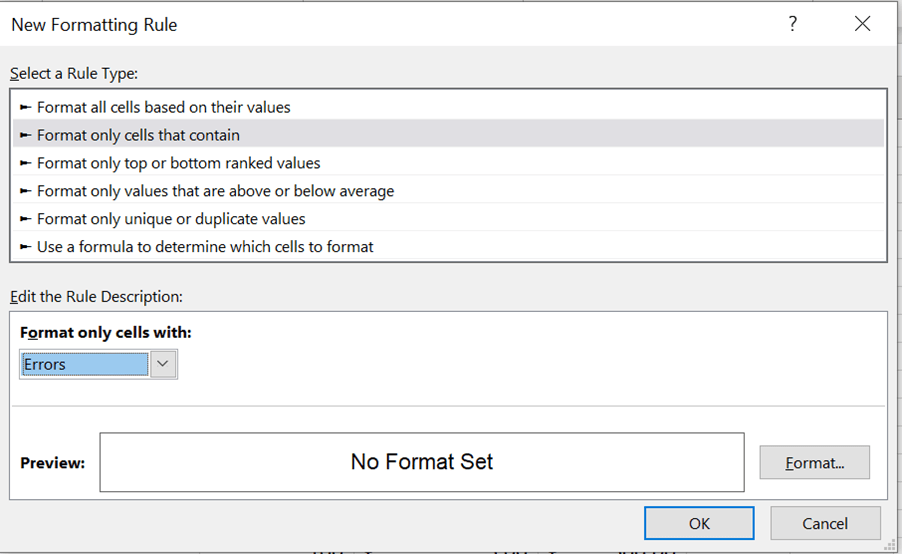
Conditional formatting can also be used to highlight errors in the worksheet. You can do this by setting up a new rule. Then, select the ‘Format only cells that contain’ rule type.From the ‘format only cells with’ dropdown select ‘Errors’:
Highlight using ‘Go To Special’
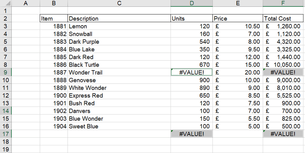
Under the ‘Find & Select’ option, we can use ‘Go To Special’ to identify and select cells with errors by selecting ‘Errors’ under ‘Formulas’.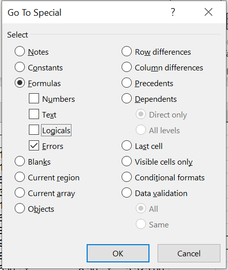
- Excel Tips and Tricks #506: Creating a single master list after merging data
- Excel Tips and Tricks #505 – 3 ways of converting US Dates into UK formats
- Excel Tips and Tricks #504 - Accessing accessibility checkers for good spreadsheet practice
- Excel Tips and Tricks #503 – Printing under pressure, super quick presentation tips
- Excel Tips and Tricks #502
Archive and Knowledge Base
This archive of Excel Community content from the ION platform will allow you to read the content of the articles but the functionality on the pages is limited. The ION search box, tags and navigation buttons on the archived pages will not work. Pages will load more slowly than a live website. You may be able to follow links to other articles but if this does not work, please return to the archive search. You can also search our Knowledge Base for access to all articles, new and archived, organised by topic.
