Excel Tips and Tricks #456 - Revisiting loan modelling

• Read TOTW #246

Excel is a powerful tool that can help to forecast the cash flow impact of differing debt terms, such as interest and tenor. This article will guide you on how to use these techniques to create your own simple loan calculation in Excel.

You will find a downloadable version of the final model at the end of this article.

In this example, we will look at a loan that we will draw on 1st July to be repaid in semi-annual instalments over the following 5 years, with an interest of 3%.

Corkscrew

This model begins by creating what is known as a “corkscrew” for the loan balance. A corkscrew can be used to track the opening and closing balance of the loan throughout the loan life to see the outstanding balance at any given point in time.

For example, in this case the opening balance plus movements in the year equal the closing balance, which is then equal to the next year’s opening balance, and so on. The dependents of each cell form a “corkscrew” shape, hence the name.

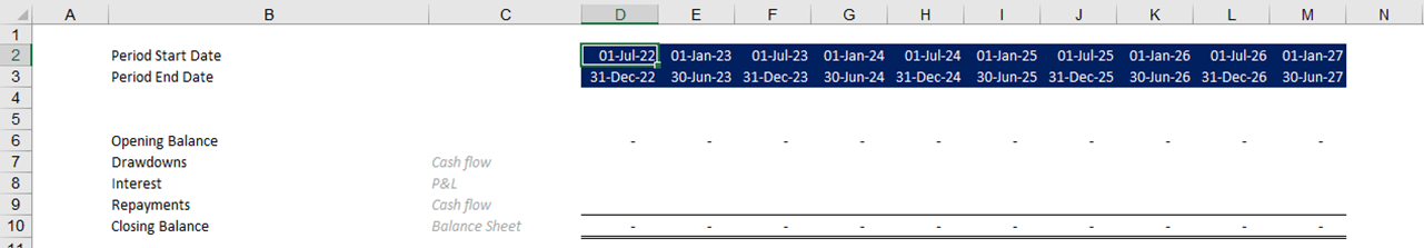
Below you will see the basis of the corkscrew of our loan, with the formulas filled out for the opening and closing balance. To make this clearer in accounting terms, you can also label each item according to its accounting entry as shown.

To avoid manual input of dates, we have used the EDATE and EOMONTH functions to populate a date for every six-month interval. This means that you only have to input the start date in cell D2 to obtain the dates over the 5-year period of the loan.

Once the basic corkscrew is set up, the next step will be to work out what the movements will be starting with the loan drawdown.

Drawdowns

This example of a simple loan has one drawdown, but it is also possible to have many.

The cells in yellow are inputs that are used to drive the formula for the “drawdown” row in the corkscrew. To make these inputs easy to identify, locate and change we can use named ranges. More information on named ranges can be found in Tip #452.

The formula can then be copied across without the need of cell anchoring ($).

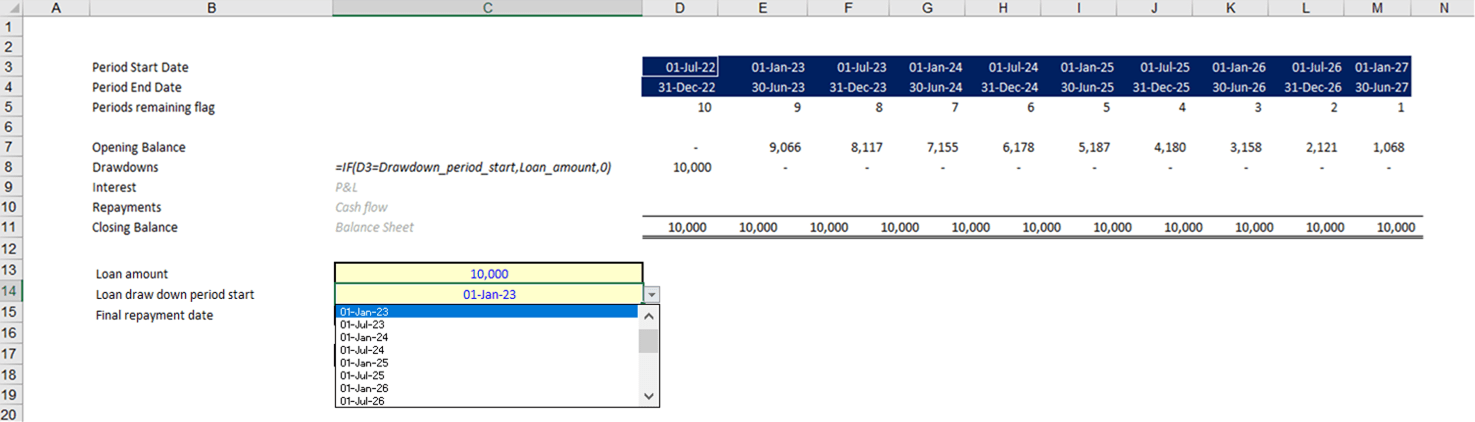
For the drawdown period start input, data validation has been used so that you are only able to select a date from the period start dates. The list of dates is linked to the dates in the template. If the dates are changed, the list will also be updated.

More information on data validation can be found in TOTW #296.

Interest calculation

In the same way as before, you can also create an input for the interest rate as this is a variable and you may want to test other rates in the future. The interest rate can also be given a named range so that it can easily be referred to in formulas.

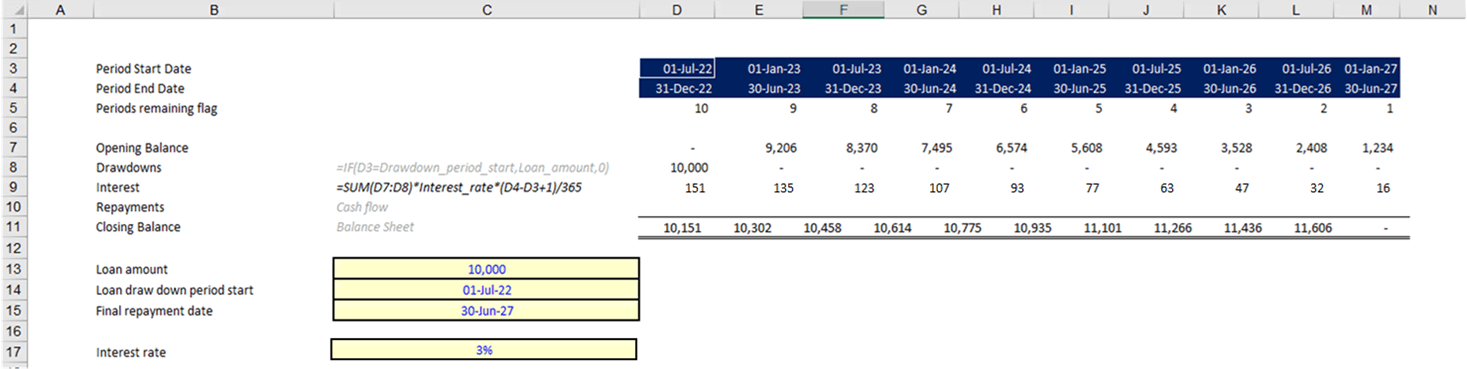
As the drawdown is happening on the first day, we have included the amount in the calculation of interest for the first period (SUM(D7:D8)).

The interest needs to be prorated to the number of days in the period. This is what the second half of the formula does (*(D4-D3+1)/365). It takes the number of days between 1 July and 31 December and works this out as a proportion of a 365-day year.

Repayment

Finally, we want to be able to calculate the repayments on the loan.

The lender could specify any method of repayment but a common one is to repay on an annuity basis.

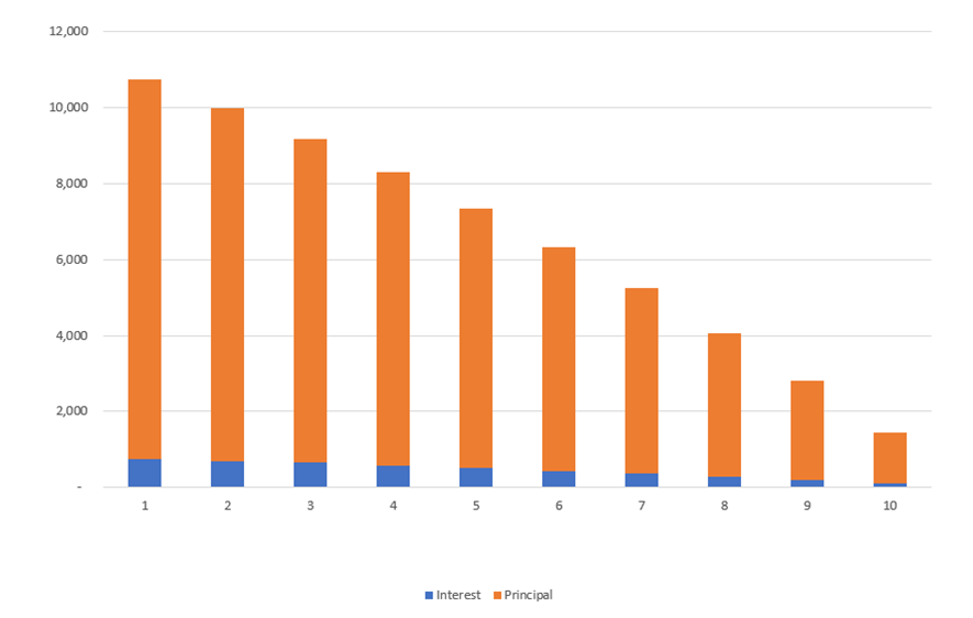
Some loans will be set up to repay a fixed amount each month, or year, and the regular payment will comprise of a proportion of interest and contribution to the loan balance. As time goes on, the ratio between interest and principal will change as demonstrated above. This visual is available in the visual tab of the template.

The PMT formula will calculate a constant repayment amount based on the interest rate and time remaining of the loan.

This may look like a complicated formula but if you break each element down, it is easily manageable:

PMT(rate,nper,pv, [fv], [type])

1. Rate – refers to the periodic loan interest rate which is the same rate we used in our interest formula.
2. Nper – refers to the number of payments for the loan. In this model, this is equal to the number of periods remaining which we have calculated using a simple formula underneath the date timeframe.
3. Pv – refers to the present value which is the loan balance (including drawdowns for the period).
4. Fv – refers to the future value of the loan. This field is optional.
5. Type – refers to the type of payment. This field is also optional.

More information on loan functions and formulas are referenced in TOTW #326.

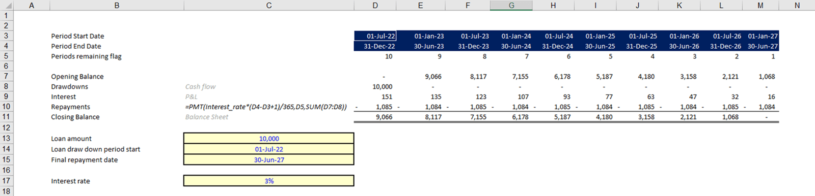
You will see that the closing balance is 0 at the end and the repayment amounts are a constant amount. The reason for the varying £1,084 and £1,805 is due to the differing lengths of each half of the year (181 and 184 days).

Changing assumptions

Because this model is set up with variable input controls, assumptions can be changed instantly if required.

For example, here is the same loan at a different interest rate, showing the higher repayments required.

And that’s your model! You can download our example workbook to see it in action.

Financial Modelling Code

Simple financial modelling in excel, such as in this example, can be useful for businesses and individuals for decision-making. For further guidance and best practice on creating financial models, you can refer to ICAEW’s Financial Modelling Code. This guidance is based on a framework of best practice for successful financial modelling.