
An introduction to ranking
There are two ranking functions in modern Excel, which function identically except for how they treat tied items – RANK.EQ and RANK.AVG.
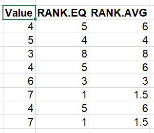
You can read more about these functions in TOTW #383, but as a reminder: RANK.EQ scores tied items with the same rank for all of them (the highest ranking in the order); RANK.AVG averages the ranks spanned by the tied items. So for example the highest two items in the above list are the two 7s – RANK.EQ ranks them both 1st before moving on to 3rd place for the one 6 in the range; RANK.AVG averages the ranks of 1 and 2 and shows each with rank 1.5.
Ranking within a group
What we want to do, however, is rank within a specific subgroup – so for example, let’s take this table of customer purchases:
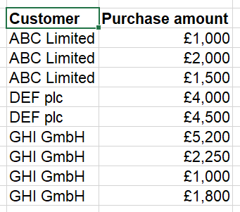
We want to rank the size of purchase by customer with a single function. How can we do this?
You might be thinking that this is analogous to functions like COUNTIFS or SUMIFS, which do familiar calculations but only considering a certain subset of the data they’re fed. What we want is essentially a RANKIFS. But that function doesn’t exist.
For several other _IFS functions that don’t exist, we can make them by using an array formula. For example, here’s a PRODUCTIFS equivalent:
=PRODUCT(IF(B3:B11="ABC Limited",C3:C11,“”))
(arrays need to be confirmed with Ctrl Shift Enter unless you’re working in Excel 365)
However, this approach doesn’t work for the two ranking functions – because these need a full list to compare the current item to, making a list with blanks for the values from the other customers returns an error. And we can’t use 0 instead of “” or similar, because 0 is an actual value and will throw out our rankings. So what can we do?
The answer is deceptively simple – we abandon the ranking functions altogether, and use COUNTIFS instead.
Ultimately, what is a ranking? It’s a count of how many items are above/below the current value. So we can use this function:
=COUNTIFS(label range, this row’s label, value range, ">"&this row’s value)+1
Note the +1 so that our ranking starts at 1 rather than at 0. You can do a reverse-ordered ranking just by flipping > to <.
Here’s the result:
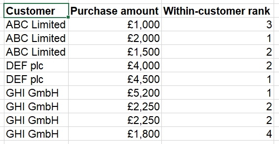
Note that this approach handles ties effectively the same way RANK.EQ does.
Related articles
Archive and Knowledge Base
This archive of Excel Community content from the ION platform will allow you to read the content of the articles but the functionality on the pages is limited. The ION search box, tags and navigation buttons on the archived pages will not work. Pages will load more slowly than a live website. You may be able to follow links to other articles but if this does not work, please return to the archive search. You can also search our Knowledge Base for access to all articles, new and archived, organised by topic.
About the author

David began his accountancy career with BDO, working for their audit team, then transitioned to the Global Outsourcing division. David joined the Excel Community Advisory Committee as a volunteer member in 2013, and started blogging for the Excel Community shortly afterwards. He is the author of the long-running series, "Excel Tip of the Week".
