Find match exceptions before they become lookup errors

We will look at using Power Query to generate lists of the products that don’t appear in both tables.

Power Query join kinds

Here are our two example tables. We will click in each in turn and use Data Ribbon tab, Get &Transform Data group, From Table/Range to load each one into the Power Query editor. Initially, we will then just use The Close & Load dropdown in the Power Query editor Home Ribbon tab to choose Close & Load to… and set the ‘load to’ location as: Only Create Connection. This makes the Table available in the Power Query editor without loading it to a Table in the workbook:

With both Tables now available in the editor, we can use Home Ribbon tab, Combine group, Merge Queries dropdown, Merge Queries as New to create a new query that combines columns from both of our Tables.

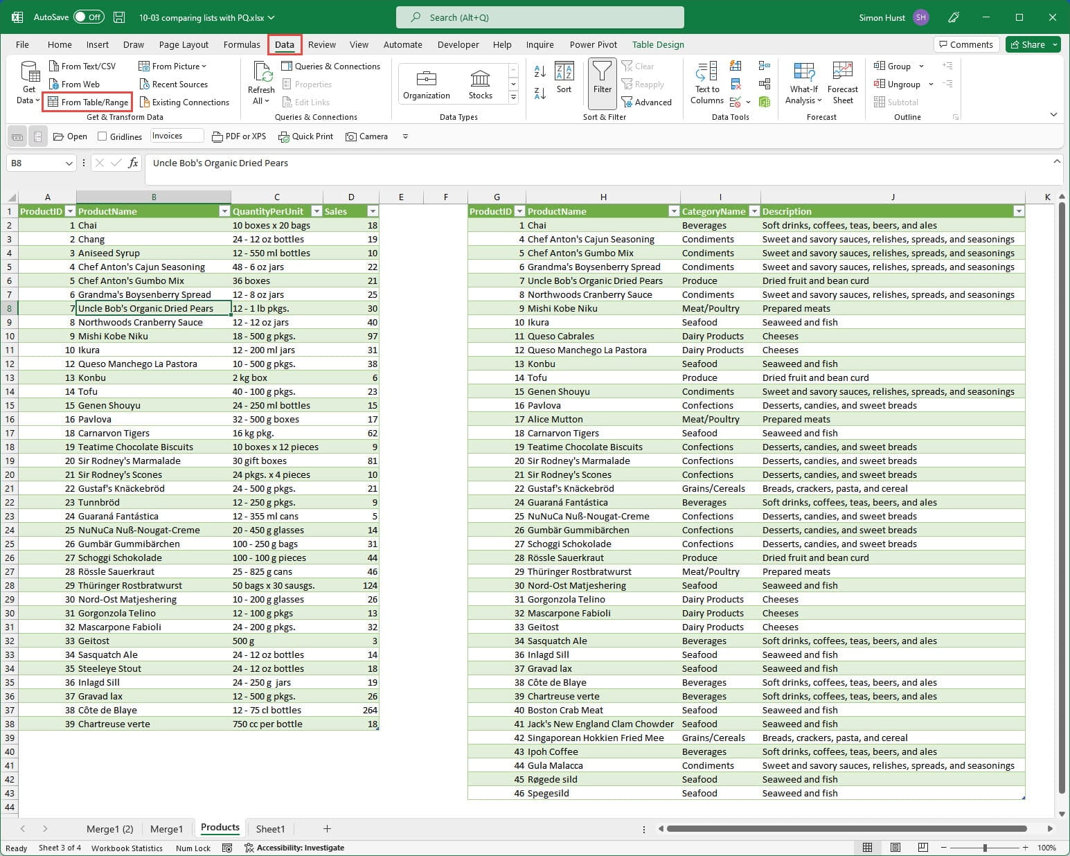
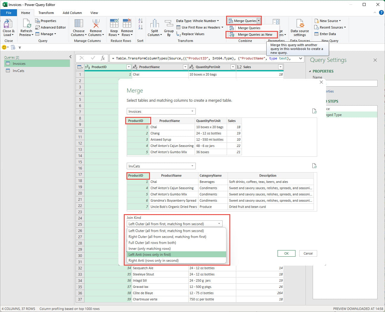
The first stage of the merge process is to choose each of our Tables in turn using the dropdowns. We then need to tell Power Query how to match our Tables. In our case, we will use the ProductID to make the match so we click on the ProductID column heading in both Tables. Note that it is also possible to match using multiple columns.

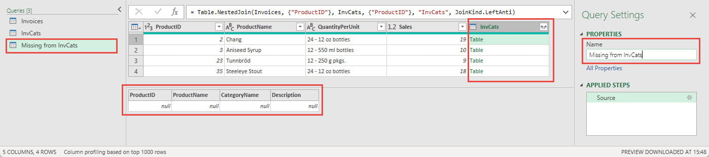
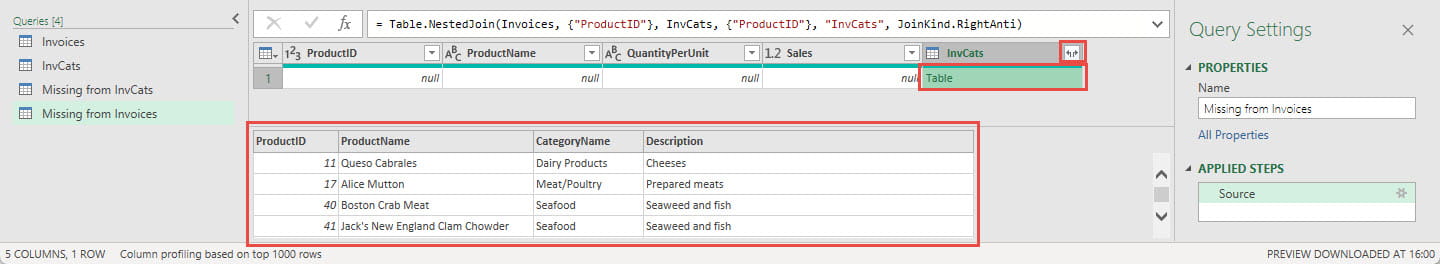
Once we have nominated our matching columns, we can choose the Join Kind from the dropdown. Usually, this is likely to be one of the Outer or Inner kinds, but we are specifically looking for items that don’t match, so we will start off by using the Left Anti join to find rows that are missing from our second Table:

Here is our resulting Table which we have renamed from Merge to the more meaningful ‘Missing from InvCats’. Each row of our Table includes, in the InvCats column, the relevant columns and rows from the InvCats Table. The rows will be empty as, by definition, there is no match in InvCats for the rows included in our merged Table. We can see this by clicking in the white space for any row in the InvCats column:

Having created a Table listing all the rows in the Invoices Table for which no match exists in InvCats, we now need to perform the check the other way round to list items that exist in InvCats but not in Invoices. The quickest way to do this is to right-click on our new merged query in the Queries pane on the left-hand side of the screen, and choose Duplicate. This creates, unsurprisingly, a copy of our existing merge query. We have renamed this new, copied, query as ‘Missing from invoices’ and clicked on the ‘gear’ symbol at the right of the Source step to re-open the merge dialog. We can then just choose the other part of our anti-join coalition, Right Anti, from our Join kind dropdown:

The result might initially be puzzling as it shows a single row of nulls. However, again this is what we should expect, as we are looking at rows that don’t exist. We still have an InvCats column, but this time the single entry holds all the columns and rows in InvCats that don’t have a match in Invoices:

To make our new query useful, we will right-click on the InvCats column heading and choose Remove Other Columns. Then we will click on the Expand/Aggregate icon to the right-hand side of the column heading and choose to expand all of our columns:

All that remains is to use Close and Load to load our Tables to an Excel worksheet where our user can review the results. We have chosen initially to use Close and Load to… to choose Only Create Connection. We have then right-clicked on each of the queries in turn in the Queries and Connections pane and chosen to load them to two adjacent Tables on the same worksheet:

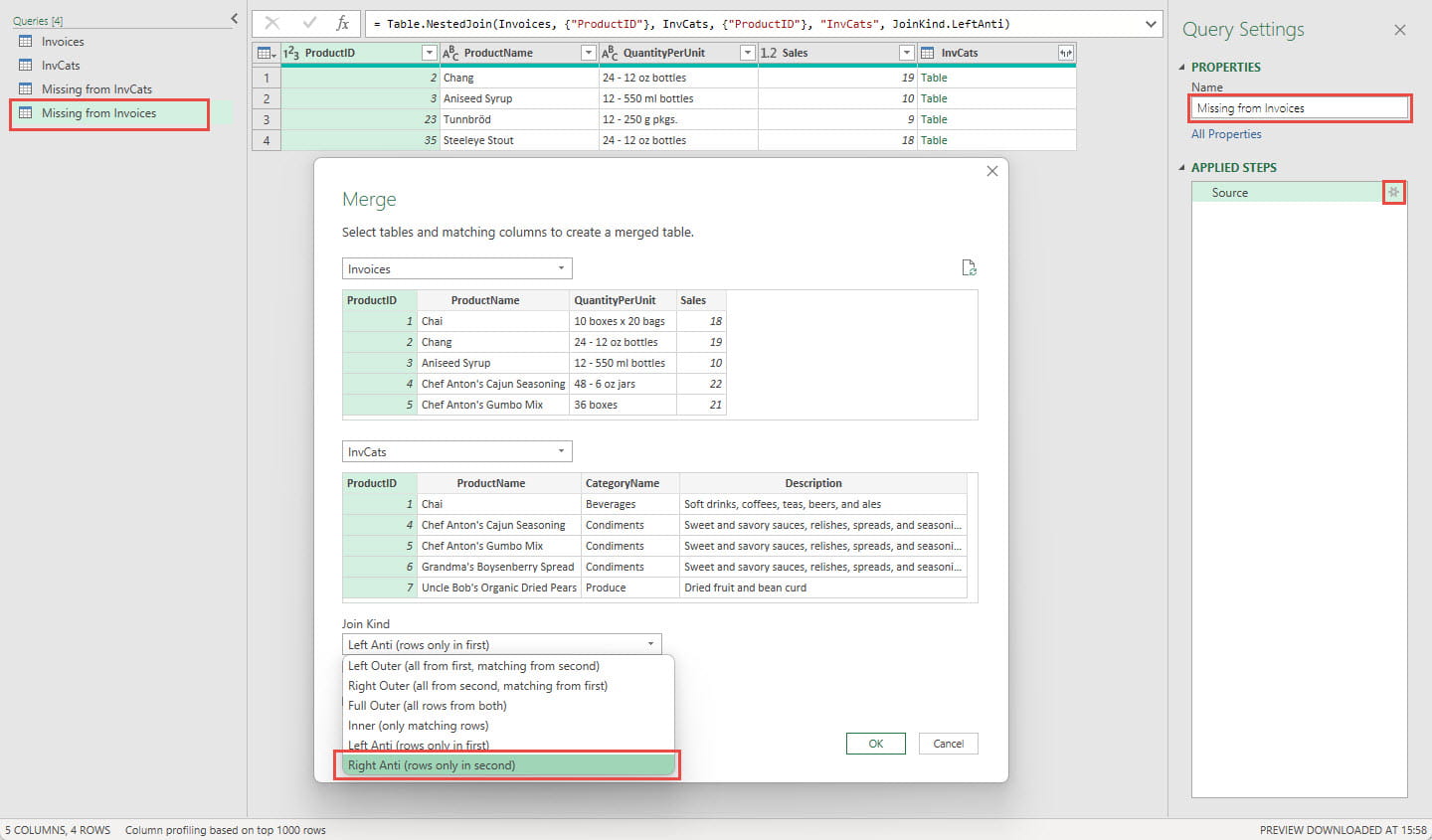
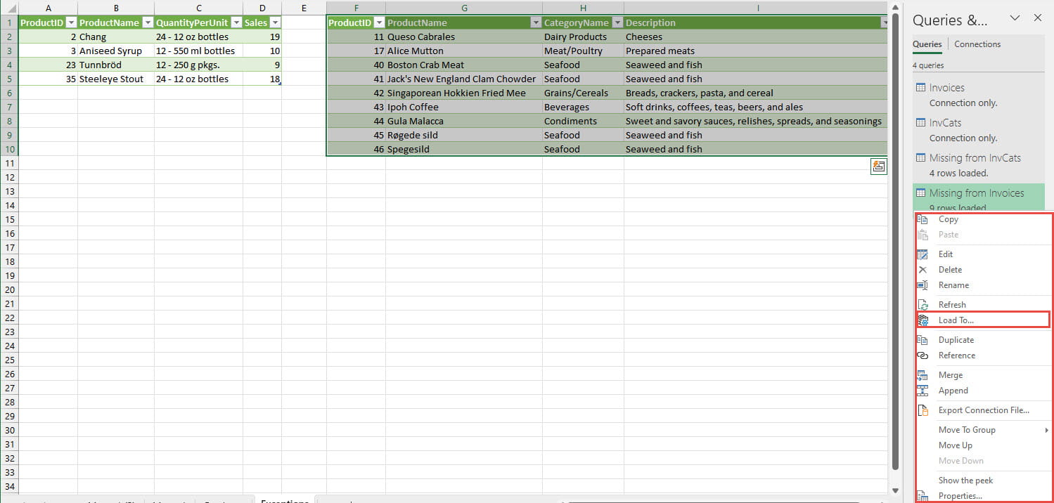
When our source Tables change, we can just refresh our exception Tables to see whether there are any unmatched items.

Related links

• Multiple Excel Tables in a single worksheet – avoiding Cell Clash
• Modern Excel - Beyond XLOOKUP. Fuzzy matching, merge & relationships