Working with Power Query Part 1: don't think cells

The structure of Power Query

As we select options from the Power Query Ribbon or the right-click menus, Power Query generates steps that apply the chosen action to our data. Each step builds on the previous step to create a revised table and the whole sequence of steps is reapplied whenever our query is refreshed. Here, we have selected a cell in an Excel Table that has the Table name 'MyData' and then chosen Data Ribbon tab, Get & Transform Data, From Table/Range to read our Table into the Power Query editor:

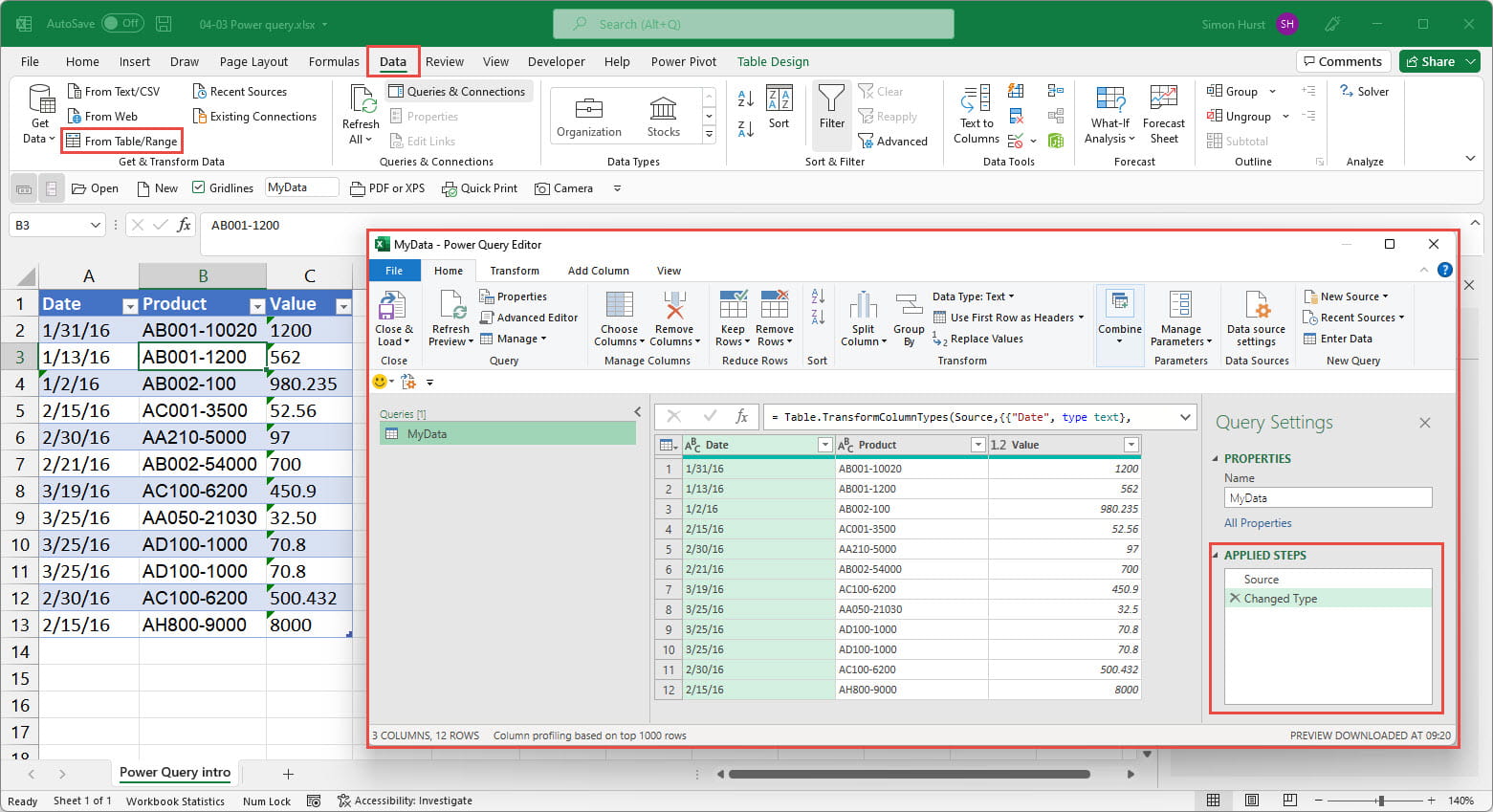
The 'From Table/Range' command opens the Power Query editor. In the Query Settings pane on the right-hand side, the APPLIED STEPS section lists the steps that Power Query has created. Although we have so far only used the single 'From Table/Range' command, Power Query has created two steps. The first step is named Source and reads the data into the editor as a Table. We can see the details of each individual step in the Formula bar. If this is not displayed, we can go to the View Ribbon tab, Layout group and select Formula Bar:

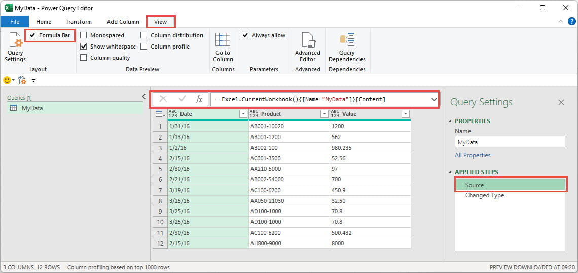
Here, we have selected our Source step in APPLIED STEPS. Our formula bar shows the line of code that brings in the content of an object called MyData from the current Excel workbook:

= Excel.CurrentWorkbook(){[Name="MyData"]}[Content]

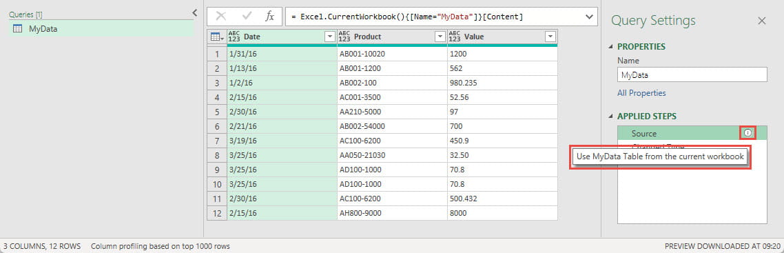
Note that you can right-click on the name of a step and select the Properties option to enter a description. This can be useful to document your process and make it easier for others to understand. For most steps you can also change the name of the step in the Properties screen or by using the Rename option in the right-click menu. If you have entered a description in this way, an information icon will appear to the right of the step name. Hovering over the step will display the description:

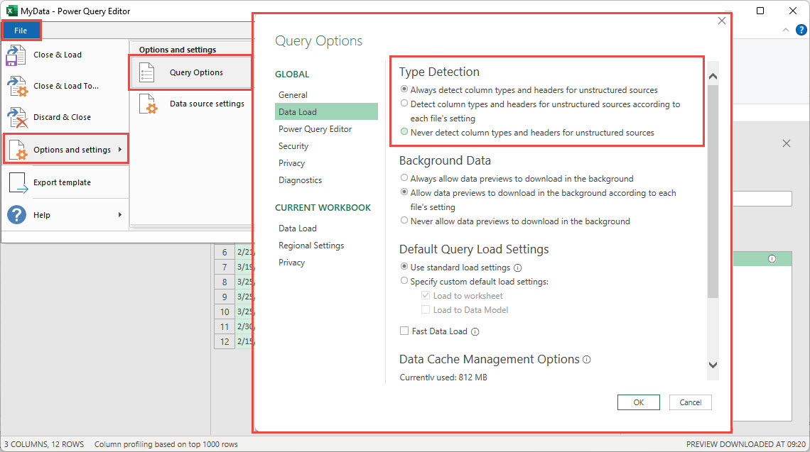
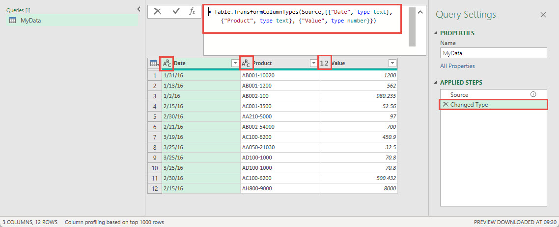
In our example, a second step has been created automatically: the Change Type step. Whether or not this step is created depends on a Power Query option. Click on File, Options and settings and then Query Options to display the different categories of options. In the Data Load category, the Type Detection options determine whether Power Query will automatically try and detect the type of data in each column and set the Data Type accordingly in a Changed Type step:

Although it is a very good idea to make sure that each of our columns does have the correct data type associated with it, do that numbers are recognised as numbers and dates as dates for example, there are some drawbacks. Firstly, we might want to set different data types to the ones that Power Query has determined and also, the automatic Changed Type step references each column by name. This can make the query less resilient to change. If someone changes the name of one of our columns in the original source data this will cause the Changed Type step to generate an error because it will reference a, now non-existent, column – even if that column is just going to be deleted in the next step. It can make more sense to delete all unwanted columns before setting our data types manually.

Again, we can click on the step in the APPLIED STEPS section to see the line of code that Power Query has created, and we can see each column referenced by name and the corresponding data types now applied to each of those columns:

We'll add another step by right-clicking in our Value column header, choosing Transform, Round, Round… and choosing to round to 2 decimal places. This is the line of code that is generated and displayed in the formula bar:

= Table.TransformColumns(#"Changed Type",{{"Value", each Number.Round(_, 2), type number}})

We can see that our new line refers to the previous, Changed Type step. Rather than thinking of this as just the previous step in the process, it can help to think of it as a table created by a step called Changed Type. This makes it clearer that a step can refer to the table created by any previous step or indeed to a table created in a range of completely different ways. For example, we can create a completely new table using a Power Query function and use this in place of the reference to our previous step:

= Table.TransformColumns(Table.FromRows({{1, 10.0945},{2, 20.535}},{"ID", "Value"}),{{"Value", each Number.Round(_, 2), type number}})

We could also refer to a separate query. Here we have created a new query that refers to the output of our original, MyData, query:

= Table.TransformColumns(MyData,{{"Value", each Number.Round(_, 2), type number}})

Conclusion

In legacy Excel, we tend to think at the level of the formula in an individual cell, even if we then copy that cell to an entire column or table. In Power Query, we can manipulate data at the level of an entire table in a single line of code. We can also refer to another table from within a table and, as we have seen, create a table within a table. One of the key advantages of thinking at the table, rather than cell, level is that our solution applies to our entire table, irrespective of the number of rows and columns we add to, or delete from, our source data. This overcomes one of the most significant problems in spreadsheets – the difficulty of dealing with unpredictable numbers of rows and columns. Of course, now that we are able to work with Dynamic Arrays in Excel, it is also possible to employ these same, table-first, thought processes within cell-based Excel.