Watch the video or read the below descriptions with updated tips.

1. First, plan your columns: it may seem like overkill but it helps. Make a list like shown here and define data types for each column. Avoid "Free type" unless necessary, like shown.

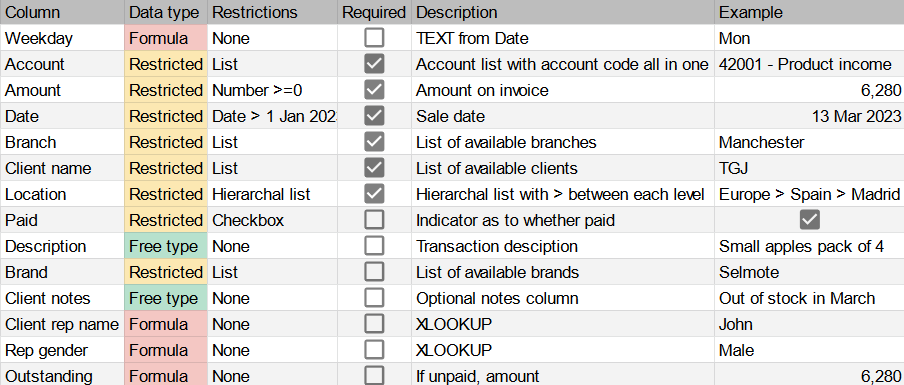
Arranging columns

2. Arrange formula columns on the far right, or occasionally far left. All data entry columns should be consecutive, otherwise people will accidentally try to type over them.
3. Signpost required columns and place adjacent. Type ! at the end of the column name to flag its importance. Google Sheets interprets * as a wildcard for search, so ! or similar is better.
4. Never merge cells inside a table. Merging gives unexpected outputs for formulas, filters, PivotTables and other commands.
5. Have one single header row. In business, multi row headers are too common (and often use the risky merged cells). They may look slightly nicer but will stop you from using many spreadsheet commands.
6. Avoid sections and subtotals. For example, if the Products column has the text "Sub-total" in one of the rows (and it is clearly not the name of the product), it contradicts the column's features. PivotTables, filters and formulas will often need to become manual.
7. Adjacent rows should be blank. Keep an entirely blank row around your table, so Google Sheets' commands (like Filter, PivotTables, Ctrl A) correctly guess table starts and ends.
8. Freeze your header row (and any important columns). Move your mouse to the column letters (A, B, C) then drag down until below the table headers.

Restricting via data validation and protection

This video shows the new updated Data Validation interface in Google Sheets:

Add your data validation by type:

9. Add date pickers. Select the column and click Data > Data validation. Then click Add rule and select "Date is on or after" (or another option) and choose "Exact date". I recommend choosing "reject the input" under "Advanced options". Cells with date validation will show a date picker on double click.
10. Add checkboxes for binary options. Select the column and click Data > Data validation, then click Add rule. In criteria, choose "Checkboxes". I recommend customising with "reject the input" again and setting Custom cell values to 0 and 1 (by doing so a SUM formula can count the ticked boxes). Note there are other ways to add checkboxes, but this route is the most flexible.

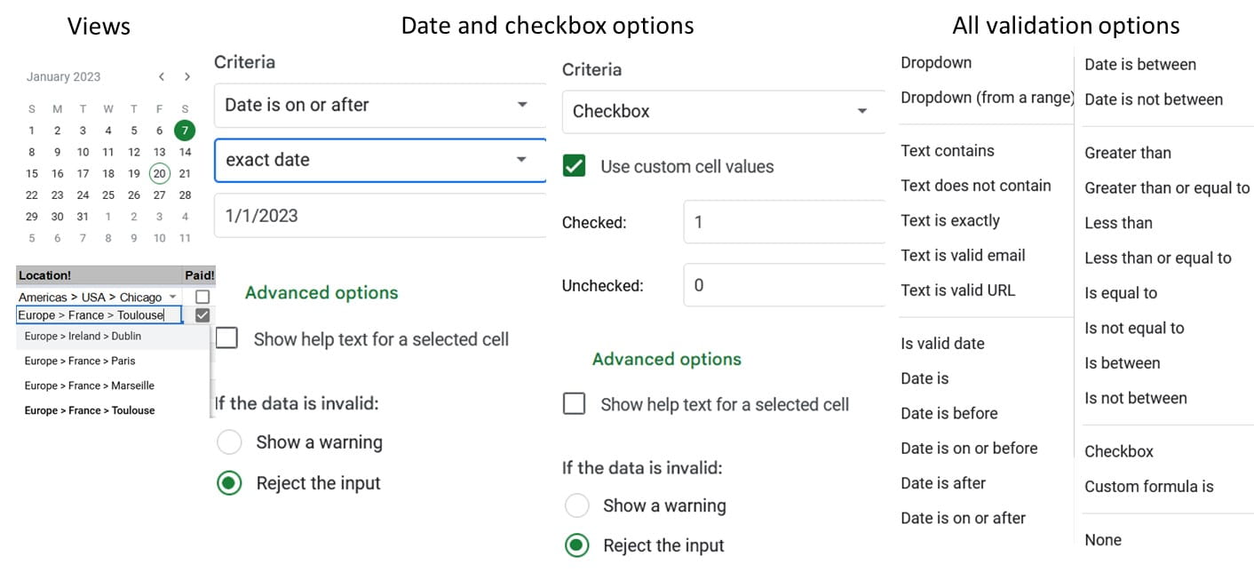
11. Validate all numerical columns. Click Add rule, select your range and then select your option. For most, I will choose "Greater than or equal to zero".
12. Single select coloured dropdowns. To add this newly enhanced feature, click Add rule and select the column. Then choose either "Dropdown" (to type options inline, colour and reorder) or "Dropdown from range" if the values are stored inside your workbook (usually on another worksheet).
    
    The latter is good practice and has a sorted list with blank entries at the end, so the list can expand for future. Google Sheets will show you autocomplete options as you type, making long dropdown lists far more efficient in Sheets than what other software offers.
    
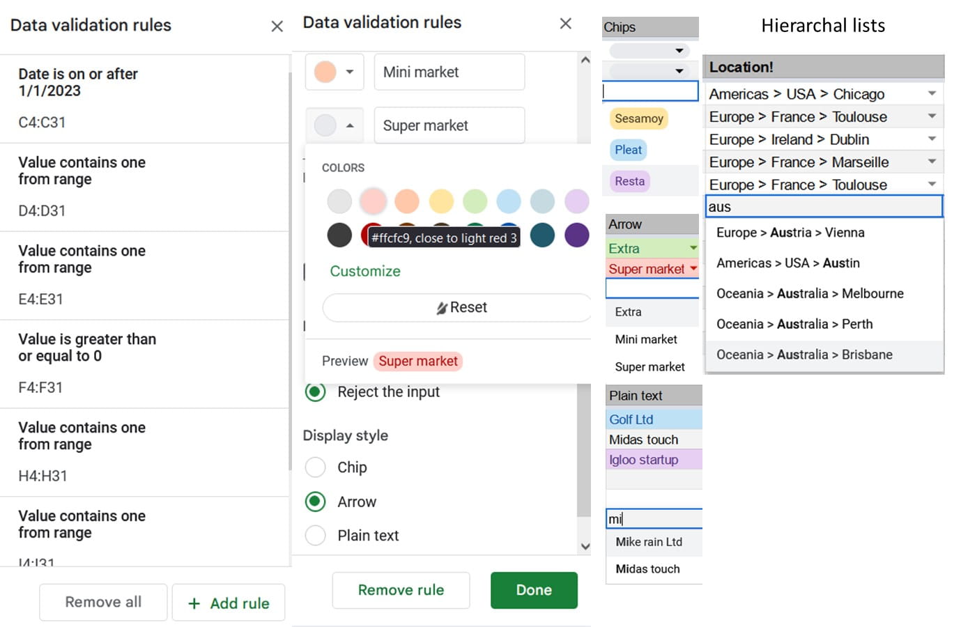
    You have three display options for dropdown with the new update:
1. Chip: an oval button, options and chosen values will be coloured. I recommend this for values with few characters only.
2. Arrow: mimicking the experience before the update, the chosen values will be coloured but not options. This is my preferred user interface.
3. Plain text: no visual marker is on the cells but use autocomplete and the chosen values will be coloured.

13. Hierarchal dropdowns: Autocomplete pops up as you type, so a dependent list could just contain entries in one cell in order or granularity. For example, when you type "Au"
    
    Oceania > Australia > Perth, Europe > Austria > Vienna and America > USA > Austin
    
    would all pop up in the list. Use arrows to toggle and press tab to lock in an entry.
    
    Autocomplete opens up other speed up opportunities; for example, "David Benaim Data > DBD > technology" is easily reachable via the full text or via the 3-letter code.
    
    A companion to hierarchal lists is:

    =SPLIT(cell, " > ",TRUE)

    At the end of the table, this splits your hierarchal value into individual columns, three in the above examples. TRUE tells Sheets that the at the split delimiter “ > ” including two space characters exactly is the split, rather than a space or a > symbol.

14. Multi select dropdowns: Without a built-in method, the best alternative is to create one column for each possibility with the same dropdown, then a formula column which combines them. TEXTJOIN (which does the opposite of TEXTSPLIT) is great for it.

    =TEXTJOIN(cell1:cellN,TRUE,“; ”)

    will combine them into a list separated by ;

The most useful part of the recent data validation upgrade though is a right-hand sidebar with a list of all the ranges which have validation applied. Remove or resize the ranges from the sidebar directly.

As before, Paste special works for Data Validation only, but unfortunately validation does not prevent people from pasting a cell with invalid data onto one with validation applied, so keep an eye every so often on whether your sidebar matches your expectation.

Protecting ranges

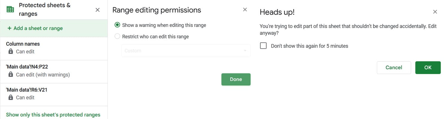
15. To lock cells, select them and click Data > Protected sheets and ranges. Choose between “Show a warning” and “restrict who can edit” where you can specify based on user. “Show a warning” is useful, as common issues come from accidental edits (and a warning would prevent them from continuing). Unfortunately, users cannot filter and sort without triggering protection warnings.

Automatic colouring

This video showcases how to automatically colour in Google Sheets:

16. Format headers at table level not cell level. The rarely used Alternating formats command allows control over header and row formatting on a table basis rather than a cell-by-cell basis, and it auto-expands when new columns or rows are added. If you're familiar with Excel's Format as Table feature, alternating colours (under the format menu) can do the same in terms of formatting (but this doesn't support Table's other features e.g. formula enhancements).
    
    Note: Always check the correct range is selected before applying.

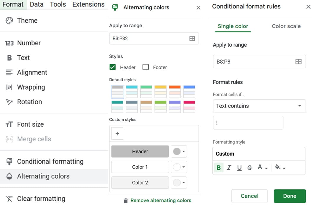
17. Bold required field names. Add an ! after each required field, and then select your header row. Select Format > Conditional formatting > Text that contains > type character, then choose OK.
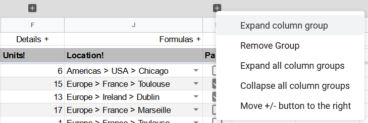
18. Group don't hide. If users should not see certain columns (or rows), select Data > Group. This makes adds a +/- expandable icon. You can add also add multiple layers or give each group a label by manually typing the group name into row 1 of the column adjacent to the + box.

Optional supporting rows, columns, and tables

19. Column instructions row: I often add a row above my table with three options (free type, formula and choose). The first is green, second red and third (which covers any validation type) in yellow. I apply the rarely used conditional formatting again for text that contains.
20. Cell count row: This counts how many entries are in each column using the function COUNTA(Column). You may choose to add an IF formula to only include it if the field is required (i.e. the last character is a ! if that is set up). Note that Column in each of these should extend well below the current range for new entries.
21. Error count row:

    ARRAYFORMULA(SUM(IF(ISERROR(Column),1,0))).

    There is no defined function for this but you can create your own functions now with Named Functions (described in further detail here).
22. Blanks count column: To count how many required entries are left blank in a row, use

    =IF(First column ="","", COUNTIFS(Current row,"",Header row,"*!")

    The *! Means the name of the column ends in ! with however many characters preceding it.
23. Check columns: Often I add check columns to check if the amount calculated in the table matches up to the amount expected, but this is computed on a case-by-case basis.

Final tip – use lookup tables

24. I usually create several lookup tables to populate my main table with two things in particular: dropdown lists and lookup values (e.g. the user must choose the product name from a dropdown, then the product price will automatically populate).
    
    I recommend the recently released XLOOKUP function which has the required fields =XLOOKUP(lookup value, lookup array, return array, described more here).

The data validation upgrade makes Google Sheets an impeccable data entry system, and with some simple tips you’ll have a robust solution.