
In this article, we talk about how to create a custom conditional formatting rule that will colour an entire row when a specific condition is met in one particular cell.
This article was originally published in 2016 as Excel Tip of the week #143.
It has been edited to reference latest Excel developments.
The issue at hand
It's pretty easy to make a rule that, for example, will turn a cell red when a certain condition occurs. It's less easy, however, to make an entire row turn red based on what one column within that row says. But it's still possible!
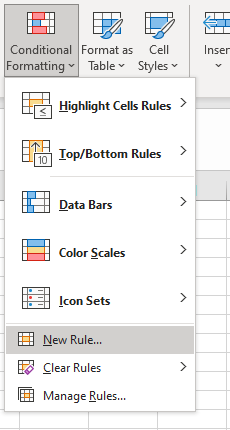
To do this, we will need to write a custom conditional formatting rule. This is done from the Home > Conditional Formatting > New Rule menu:
The specific option you need is the bottom one:
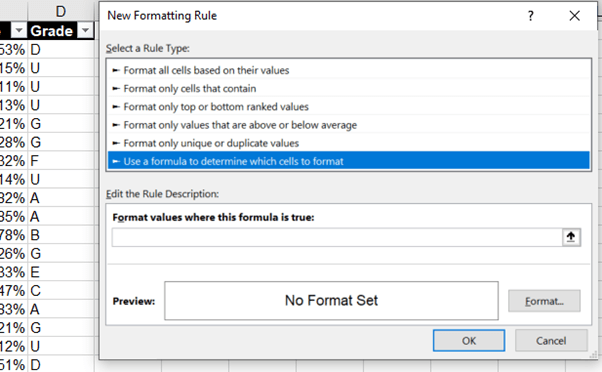
What we need to write here is a formula that will produce a TRUE/FALSE result - like the ones covered in Tip #273 as the first input of an IF function. The formula will be interpreted from the perspective of the active cell when the dialogue box is opened; in this case that is cell D2. It's important to use fixed references (Tip #200) carefully to get the desired results.
The example I will use is a grading table for a set of exams. (You can download the example file here). We want each row to turn red if a U grade has been assessed for a particular student. So, the formula we need is:
=$D2="U"
This rule uses a dollar-sign to fix column D. This means that, wherever the conditional formatting rule is applied, it will check Column D for its result. However, the number 2 - the row number - has no dollar and will be different across each row of the table as appropriate.
You can inspect this formula in the example file, by selecting the table and navigating to Conditional Formatting > Manage Rules.
We can also write more complicated functions. For example, we can highlight any student that scored an A or A* grade:
=OR($D2="A",$D2="A*")
Another example would be highlighting the top three scores on each individual paper (written from perspective of cell C5):
=RANK.EQ(C2,C$2:C$21)<=3
You can apply this logic to create almost any custom rule you desire. However, the input box for the rules does not show the tooltip for any functions you write and can be fiddly to use. It's often better to write the function in a cell directly whilst you're developing it, and then cut and paste the formula text into the conditional formatting menu once you're happy with it.
Archive and Knowledge Base
This archive of Excel Community content from the ION platform will allow you to read the content of the articles but the functionality on the pages is limited. The ION search box, tags and navigation buttons on the archived pages will not work. Pages will load more slowly than a live website. You may be able to follow links to other articles but if this does not work, please return to the archive search. You can also search our Knowledge Base for access to all articles, new and archived, organised by topic.
