INDEX and MATCH

INDEX and MATCH – as a combination – are two of the most useful functions at a modeller’s disposal. They provide a versatile lookup in a way that LOOKUP, HLOOKUP and VLOOKUP simply cannot. The best way to illustrate this point is by means of an example. For those thinking about XLOOKUP, don’t worry, I will mention this function again in a later blog!

Here is a common problem. Imagine you have built a financial model and your Balance Sheet – ahem! – contains misbalances. You need to fix it. Now I am sure you have never had this mistake yourself, but you have “close friends” that have encountered this feast of fun: solving Balance Sheet errors can take a long while. One of the first things modellers will do is locate the first period (in ascending order) that has such an error, as identifying the issue in this period may often solve the problem for all periods. Consider the following example:

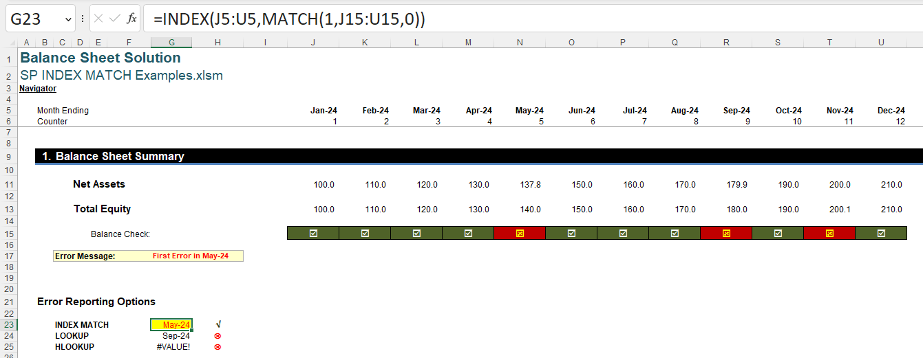
This is a common modelling query. The usual suspects, LOOKUP and HLOOKUP / VLOOKUP do not work here:

• LOOKUP(lookup_value, lookup_vector, [result_vector]) gives the wrong date as the balance checks are not in strict ascending order (i.e. ascending alphanumerically with no duplicates); whilst
• HLOOKUP(lookup_value, table_array, row_index_number, [range_lookup]) gives #VALUE! since the first row must contain the data to be ‘looked up’, but the Balance Check is in row 15 in our example above, whereas the dates we need to return are in row 5 – hence we get a syntax error.

There is a solution, however: INDEX MATCH. They form a highly versatile tag team, but are worth introducing individually.

Essentially, INDEX(array, row_number, [column_number]) returns a value or the reference to a value from within a table or range (list). For example, INDEX({7,8,9,10,11,12},3) returns the third item in the list {7, 8, 9, 10, 11, 12}, i.e. 9. This could have been a range: INDEX(A1:A10,5) gives the value in cell A5, etc.
INDEX can work in two dimensions as well (hence the column_number reference). Consider the following example:

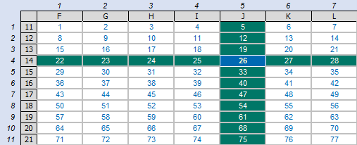
INDEX(F11:L21,4,5) returns the value in the fourth row, fifth column of the table array F11:L21 (clearly 26 in the above illustration).

MATCH(lookup_value, lookup_vector, [match_type]) returns the relative position of an item in an array that (approximately) matches a specified value. It is not case sensitive.

The third argument, match_type, does not have to be entered, but for many situations, I strongly recommend that it is specified. It allows one of three values:

• match_type 1 [default if omitted]: finds the largest value less than or equal to the lookup_value – but the lookup_vector must be in strict ascending order, limiting flexibility;
• match_type 0: probably the most useful setting, MATCH will find the position of the first value that matches lookup_value exactly. The lookup_array can have data in any order and even allows duplicates; and
• match type -1: finds the smallest value greater than or equal to the lookup_value – but the lookup_array must be in strict descending order, again limiting flexibility.

When using MATCH, if there is no (approximate) match, #N/A is returned (this may also occur if data is not correctly sorted depending upon match_type).

MATCH is fairly straightforward to use:

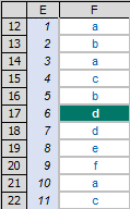
In the figure above, MATCH(“d”,F12:F22,0) gives a value of 6, being the relative position of the first ‘d’ in the range. Note that having match_type zero [0] here is important. The data contains duplicates and is not sorted alphanumerically. Consequently, using match_type 1 and -1 would give the wrong answer: 7 and #N/A respectively.

Whilst useful functions in their own right, combined they form a highly versatile partnership. Consider the original problem:

MATCH(1,J15:U15,0) equals 5, i.e. the first period the balance sheet does not balance in is Period 5. But we can do better than that. INDEX(J5:U5,5) equals May-24, so combining the two functions:

=INDEX(J5:U5,MATCH(1,J15:U15,0))

equals May-24 in one step. This process of stepping out two calculations and then inserting one into another is often referred to as “staggered development”. No, this is not how you construct a financial model late in the evening after having the odd drink or two!

Do note how flexible this combination really is. We do not need to specify an order for the lookup range, we can have duplicates and the value to be returned does not have to be in a row / column below / to the right of the lookup range (indeed, it can be in another workbook never mind another worksheet!). With a little practice, the above technique can be extended to match items on a case sensitive basis, use multiple criteria and even ‘grade’. The attached Excel file provides further examples.