Get your errors right

Error checking functions

Sometimes, when creating a workbook, you will want an Excel formula to return a particular result, rather than the default error message, should the formula return an error. A common example would be the calculation of a variance when the divisor is zero, so that the formula would return a #DIV/0! Error. In this case, it would be possible to use a simple IF() function to handle the error and return a chosen value, or a suitable text warning:

=IF(B2=0,0,A2/B2)

In this case, we can easily predict and identify the situation that we want to allow for, and create a formula that will avoid using the formula that causes the error in the first place. However, sometimes we will need our formula to be evaluated before we know that there will be an error. In these cases, we can use one of Excel’s error checking functions to check the value that our formula will return. We will work through the possible functions from the oldest to the most recent.

ISERROR(), ISNA(), ISERR()

The range of IS… functions allows you to see whether the result of a formula satisfies a particular criterion such as being an even number - ISEVEN(), or an odd number – ISODD(). The functions return the Boolean values TRUE or FALSE depending on whether the criterion is met or not.

Three of the IS… functions relate to errors. ISERROR() returns TRUE if the formula evaluates to any error; ISNA() returns TRUE if the formula evaluates to an #N/A error and ISERR() returns TRUE if the formula evaluates to any error other than #N/A:

Because these functions return TRUE or FALSE, we can use them as the first argument of an IF() function to return a particular value or text string when an error occurs:

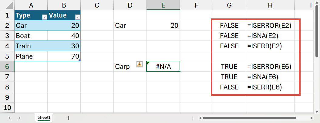
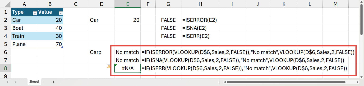
In these three formulas, ISERROR() and ISNA() both return TRUE as the formula returns is an #N/A error, so the IF() functions return the second, value if true, argument. ISERR() doesn’t return an error for #N/A errors, so the third, value if false, argument is returned which is our formula that returns the #N/A error.

The danger of using ISERROR() rather than the more specific ISNA() function is that ISERROR() will return TRUE for any error, so if there was a valid match, but there was some other error, such as a spelling error in the function name, the formula would still evaluate as TRUE and return the “No match” text:

As you can see, only the ISNA() function allows the actual error to be correctly identified. The other two functions display ‘No match’ even though there is a match. The situation would probably be even more serious if we decided that the failure to return a match should simply return 0. ISERROR() and ISERR() would just ‘silently’ return the wrong answer if the actual error were to be anything other than an #N/A error:

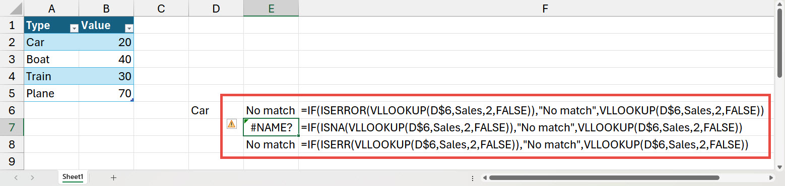
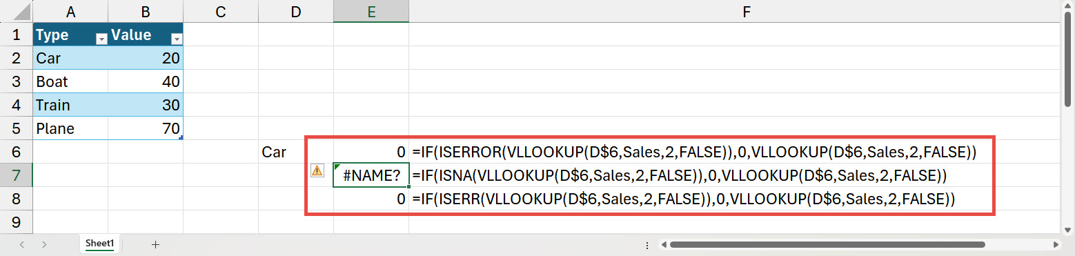
Hopefully, this shows how important it is to choose the correct, and usually most specific, error check function.

ERROR.TYPE()

It is possible to be even more specific than just choosing ISNA() rather than ISERROR(). The ERROR.TYPE() function returns a number that represents the different error types possible:

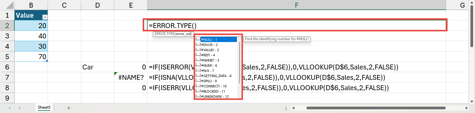
We could use ERROR.TYPE() to provide very specific warning messages based on these return values:

=IF(ERROR.TYPE(E7)=5,"Please check the spelling in the formula","Other error")

IFERROR(), IFNA()

Using the IF() function with the IS… functions requires the formula to be entered twice: once to see if it generates an error and then to return the actual result if it doesn’t. More recent versions of Excel include two additional functions that simplify the formula. Both IFERROR() and IFNA() take two arguments: the formula to be evaluated and the value to return if it evaluates to the chosen error. If it doesn’t evaluate to the error, the function will return the result of the formula without it needing to be added a second time:

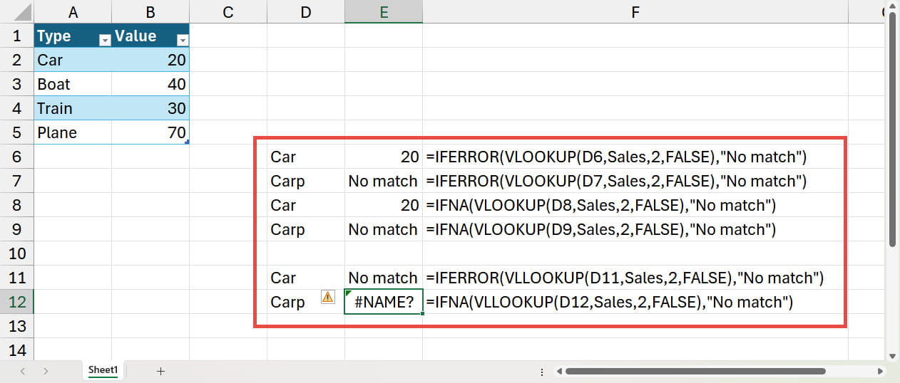
Again, we can see the importance of using the more specific IFNA() version of the function.

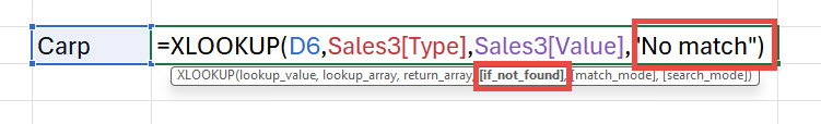
XLOOKUP()

We have used VLOOKUP() for our examples of the failure to find a match. In recent versions of Excel, VLOOKUP() has been replaced by the much-enhanced XLOOKUP() function. One of the many benefits of the use of XLOOKUP() compared to the functions that it has replaced is its inclusion of a specific argument to deal with the failure to find a match:

Conclusion

You can explore many of the various techniques we have covered here, and a great deal more, in the ICAEW archive