
Hello all and welcome back to the Excel Tip of the Week! This week we have a General User post in which we’re diving back in to a topic for a definitive revisit – the Subtotal feature.
This was last covered back in TOTW #160, and is not to be confused with the related SUBTOTAL function, which you can read about in TOTW #151.
What does the Subtotal feature do?
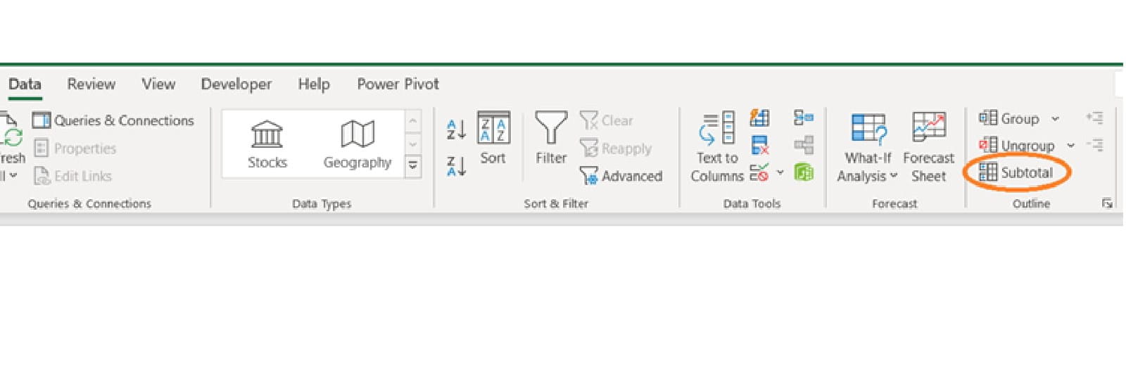
This is a button that forms part of the Data => Outline group on the Ribbon:
This feature can automatically create a grouped summary of data. The end result is similar to a PivotTable, except instead of creating a separate, linked summary, Subtotal keeps the data where it is and inserts subtotal figures and grouped rows to create an expandable, multi-level summary. It inserts formulas as it goes to make the whole thing hang together.
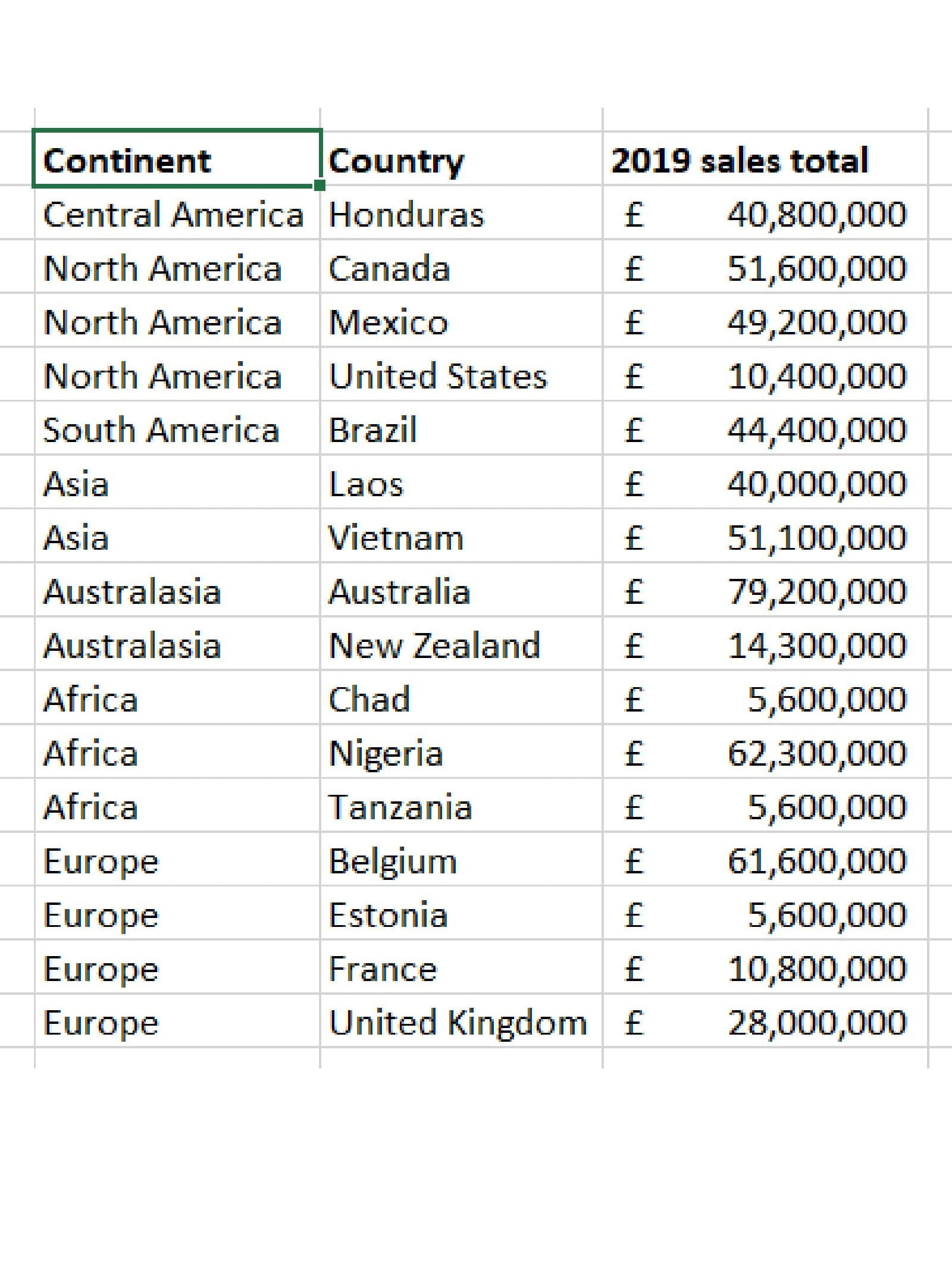
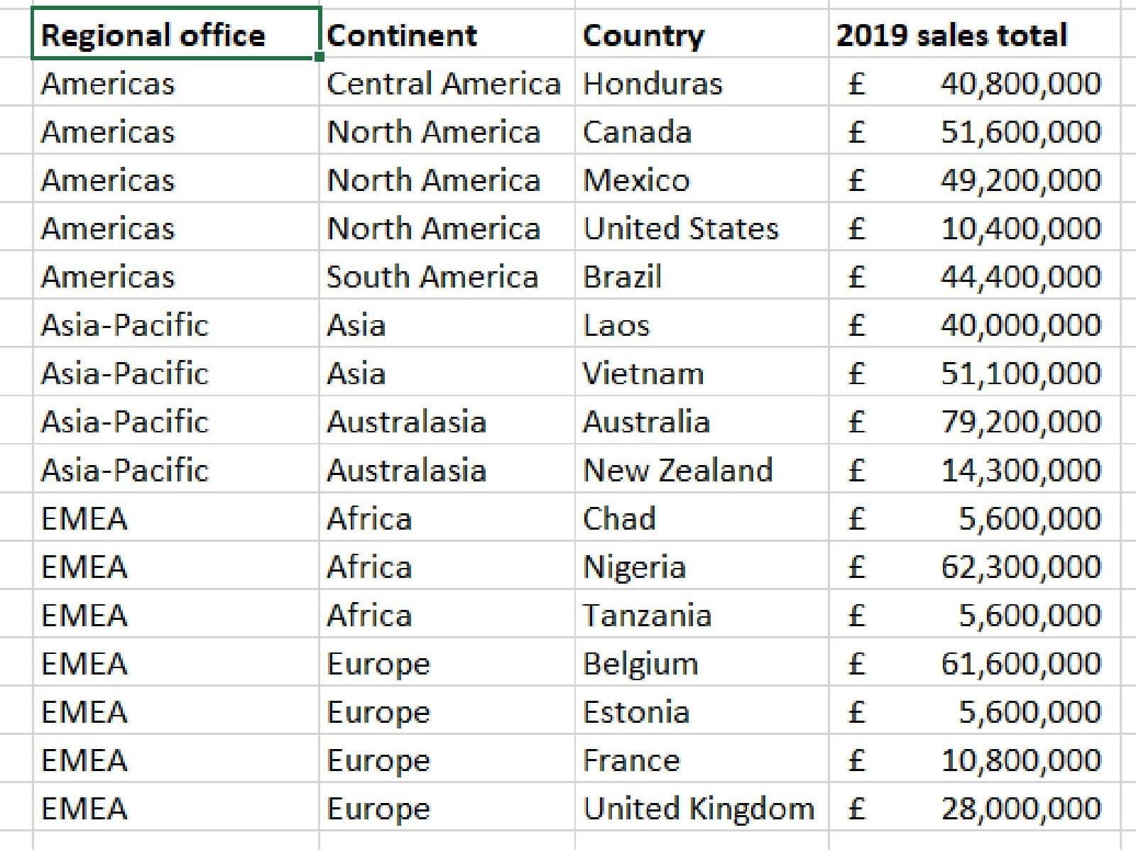
Here’s a simple example – we have a breakdown of 2019 annual sales figures by country and by continent:
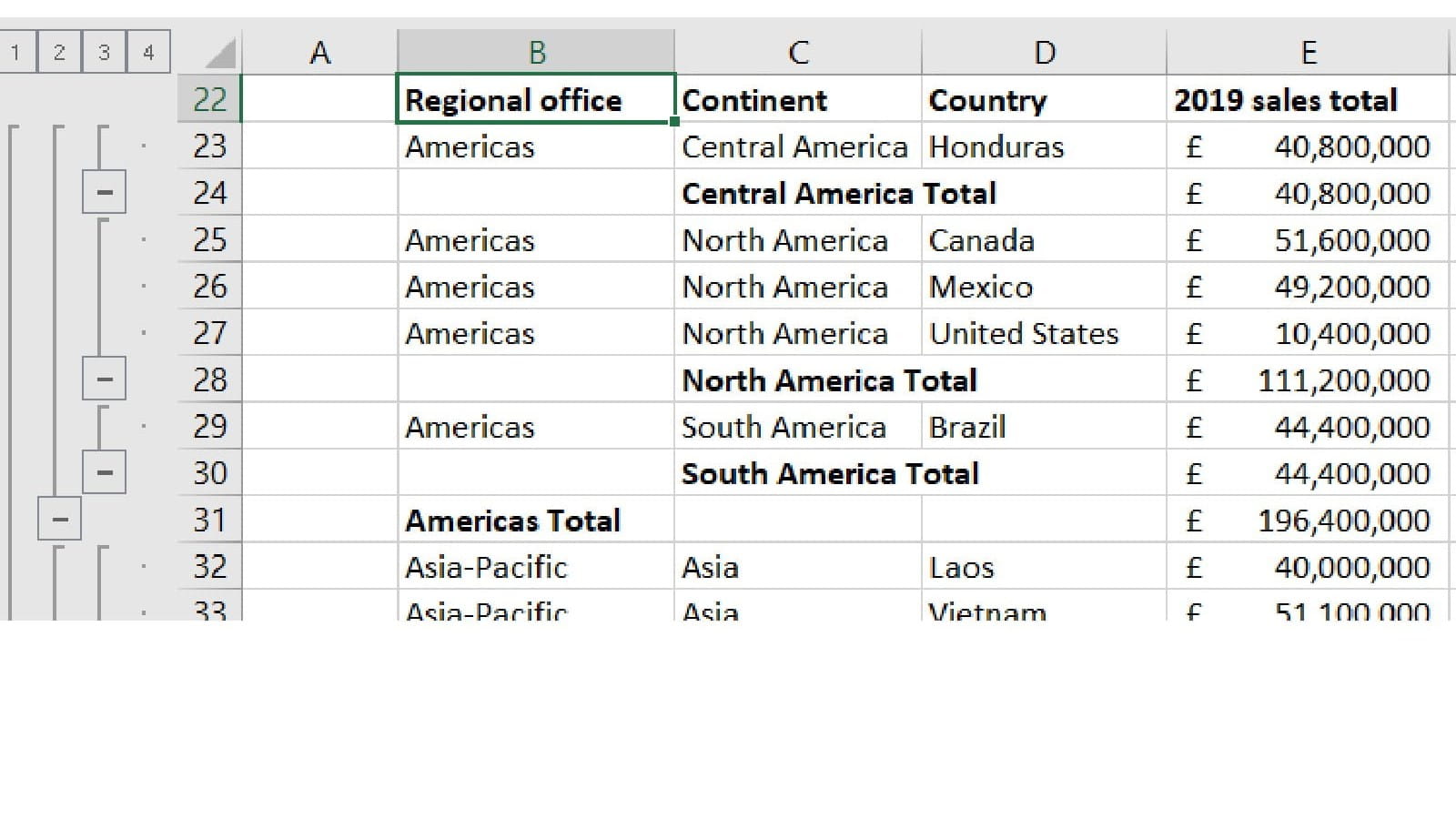
And here’s the resulting Subtotal result:
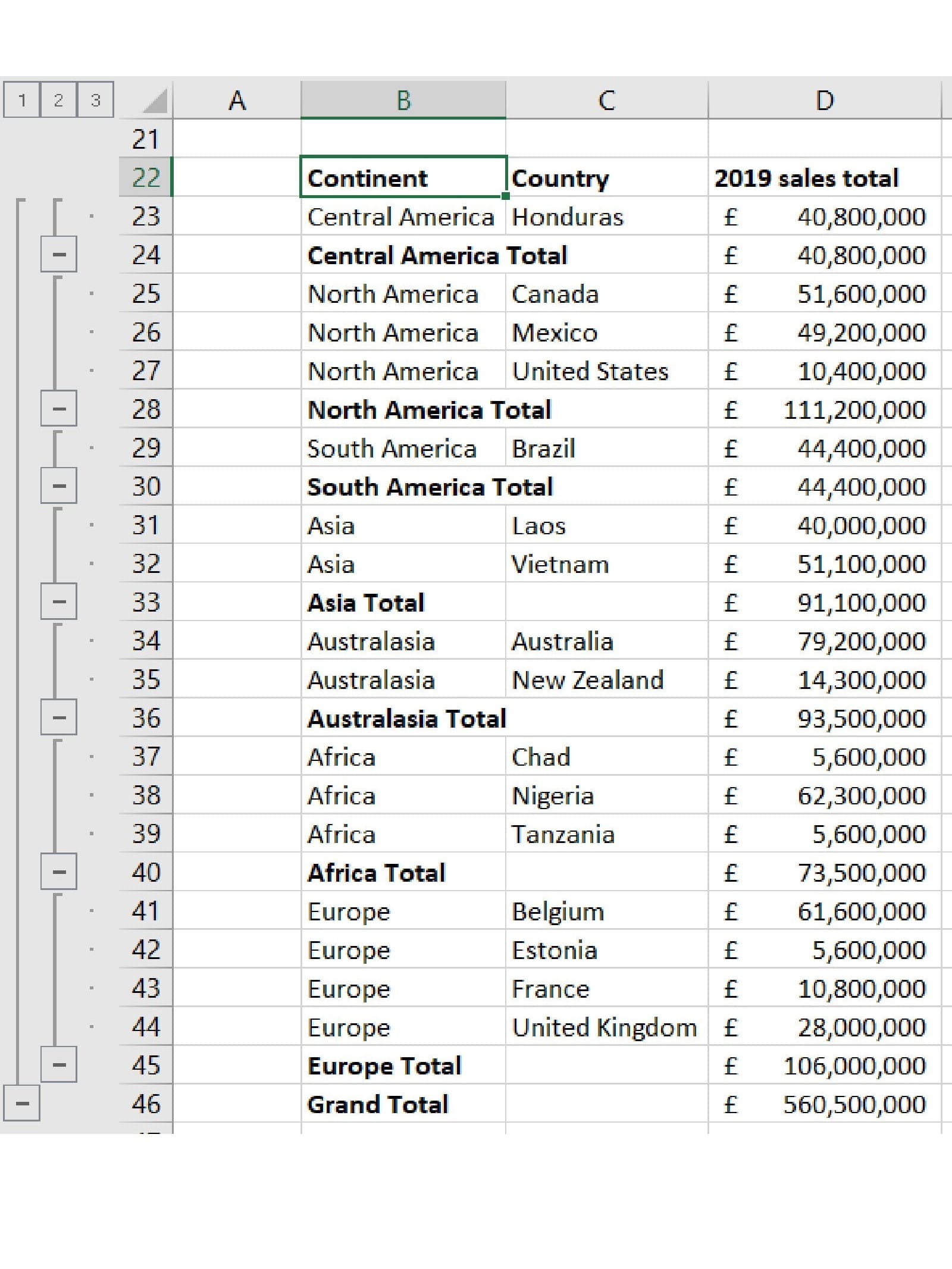
The total rows are automatically inserted, and the formulas in them only add the corresponding items from the preceding section. The Group labels at the left can be used to expand & collapse each continent individually, or the 1/2/3 buttons at the top can be used to collapse to either only the Grand Total, the Continent-level totals, or the full detail as seen here.
How to apply subtotals
Your data needs to be laid out as seen in the “before” screenshot above – with a header row and sorted so that all the items you want grouped together are listed sequentially. If you don’t sort your data first, each bubble of like continents gets their own separate total!
Then we click the Subtotal button and get this menu:
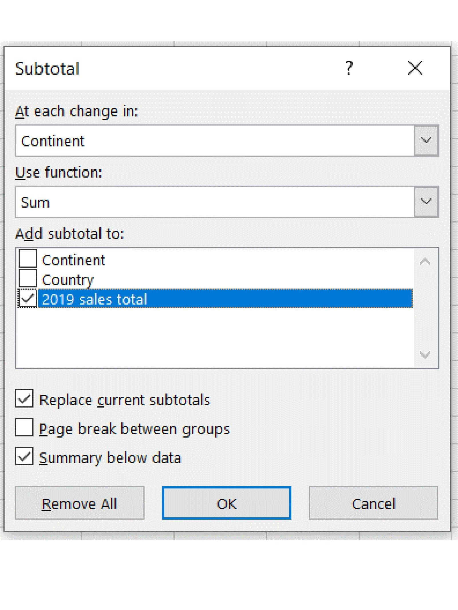
Note that Excel automatically detects the header row (the first row) and then uses the labels from that row to make for easier reading.
The menu is pretty straightforward – we indicate which column we want to group first, then select what kind of total we want to use (almost always sum, but options such as count or average are also available), and then note which column should be used for making those totals.
Before we move all, also note that there’s a Remove All button here if you later want to revert the data to just the flat table layout.
More complex examples
You can actually make more complex versions by using the Subtotal feature more than once. Let’s continue our previous example but add a “regional office” column that groups the continents together into Asia-Pacific, EMEA, and Americas. We then re-sort the data to once again get everything grouped together:
To get our finished product, we just do our subtotal process twice – first for the Regional office column, then for the Continents. And hey presto:
You can see the before-and-after versions of both datasets in the example file, available here.
You may also like
Archive and Knowledge Base
This archive of Excel Community content from the ION platform will allow you to read the content of the articles but the functionality on the pages is limited. The ION search box, tags and navigation buttons on the archived pages will not work. Pages will load more slowly than a live website. You may be able to follow links to other articles but if this does not work, please return to the archive search. You can also search our Knowledge Base for access to all articles, new and archived, organised by topic.
