
Hello all and welcome back to the Excel Tip of the Week. This week we have a Creator level post in which we’re taking a definitive revisit to the handy data transformation tool, Text to Columns.
What is this feature all about? How do you use it?
Text to Columns is a very long-standing data transformation tool that can help parse data in one column and separate it into several. It’s particularly commonly used when dealing with data imported from other programs, for example comma-separated values.
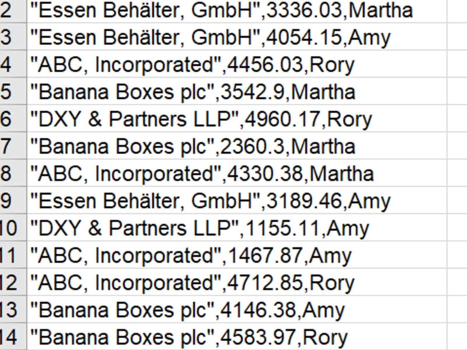
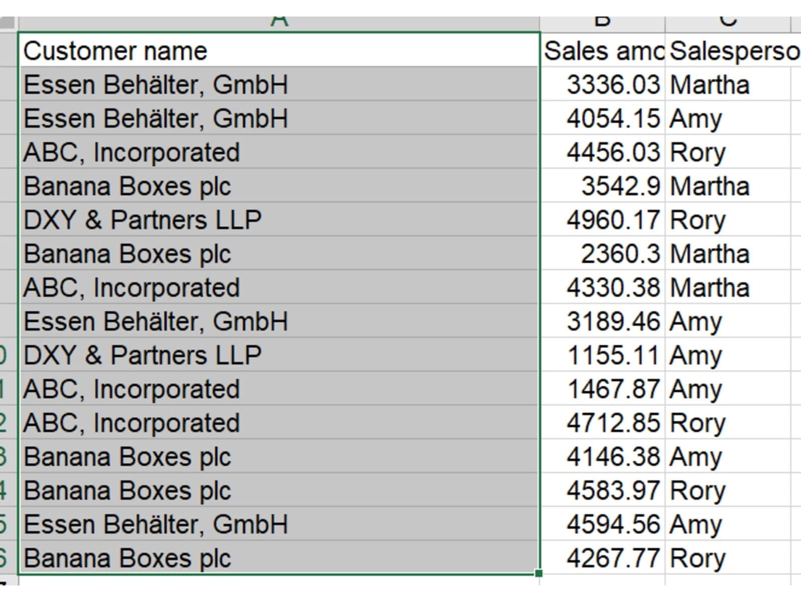
For an example, let’s take a look at this sample sales data:
We can convert this single-column data by selecting it and then using the Text to Columns Wizard, which is accessed from Data => Text to Columns:
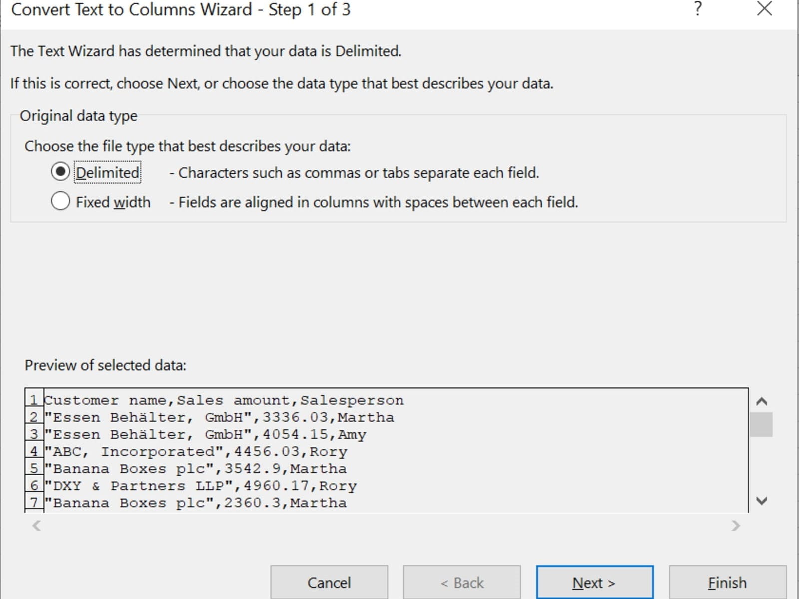
The options here are for how the new columns will be created – “Delimited” means that each column is marked by some particular character, and “Fixed width” is for cases where the data has been lined up visually and essentially needs cutting into strips. Here we are dealing with delimited data.
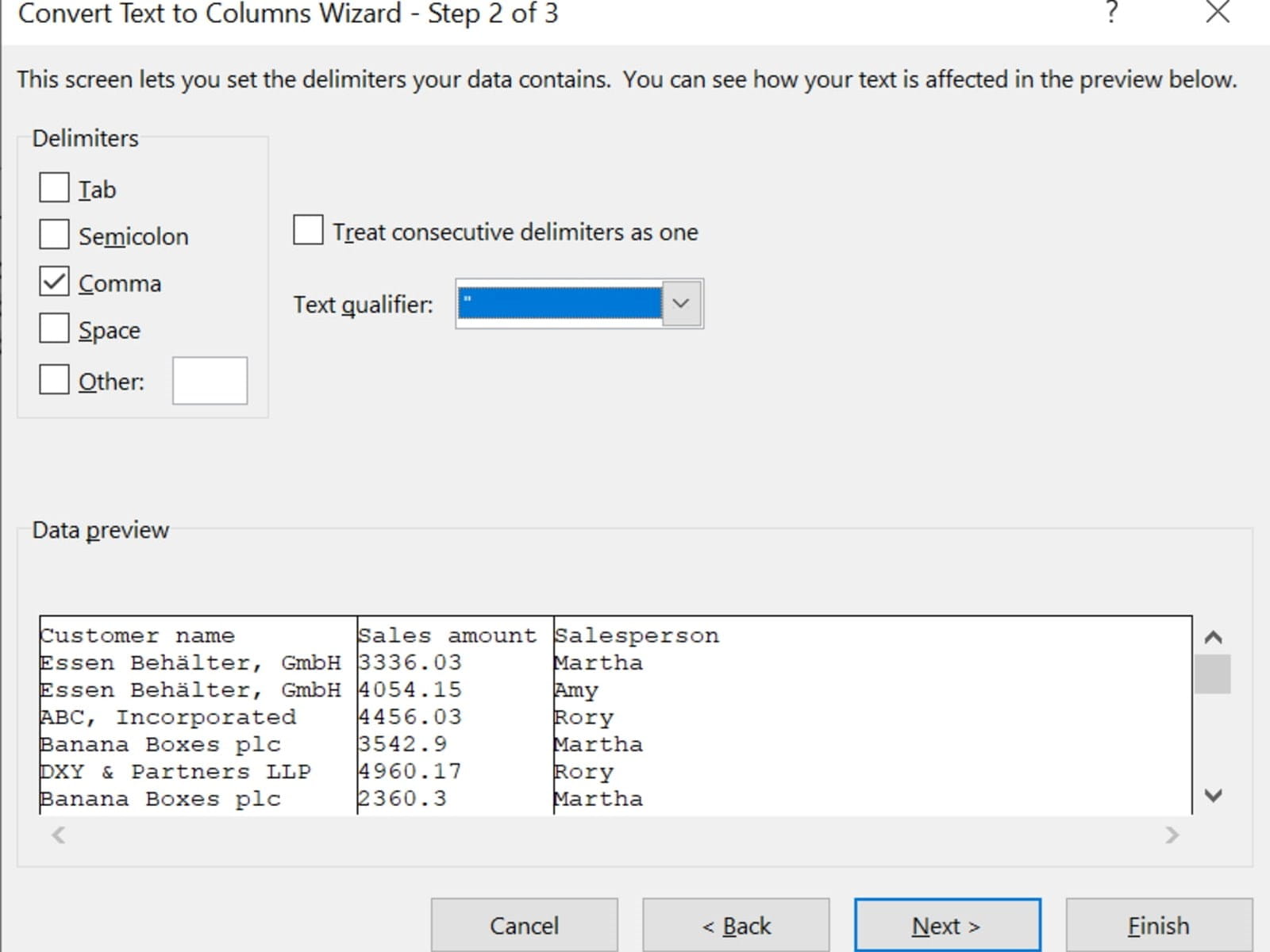
On the left here we can see where we identify which character is the delimiter. A selection of common options is given, or we can specify our own. This example also shows us how we can use the “text qualifier” field: In our original data, some of the customer names – e.g. ABC, Incorporated – include commas. Normally this would cause a problem, as the two parts of the name would get separated – but in our case, the customer names are all wrapped in quotation marks. By setting the quotation makes as a text qualifier, we can tell Excel to ignore any delimiter characters between them. We can see in the live preview that this will get us the result we want.
Most of the time you can just stop here and press Finish, but for completeness’ sake here’s the final step in the Wizard:
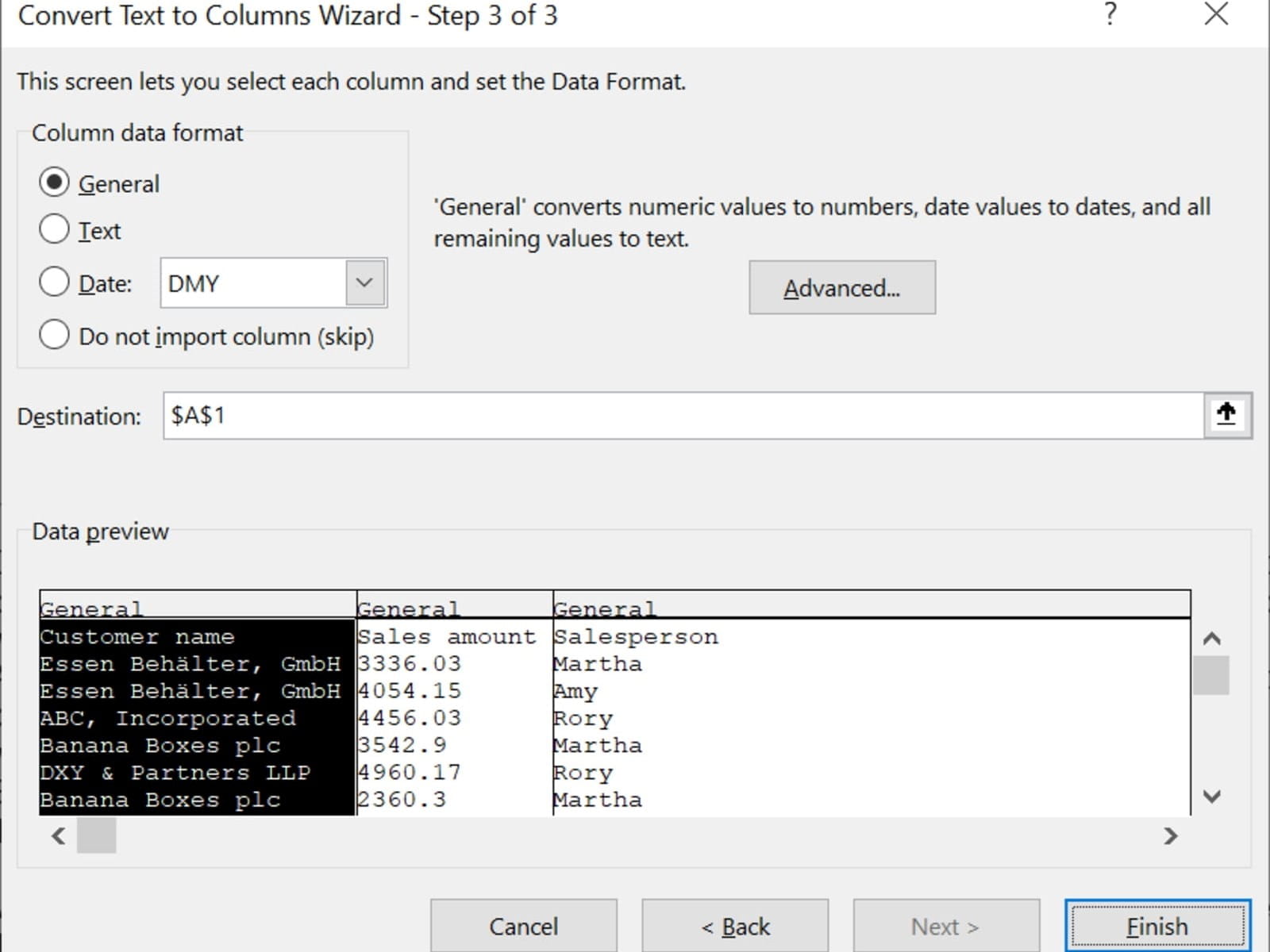
If you do use this step, you can specify a format for each new column that will be created. You can also use the “Destination” box to specify a location for the new columns – by default they are placed over the top of the original data, overwriting it, but if you prefer you can place them elsewhere and retain the original data as well.
The Advanced option here is interesting to consider:
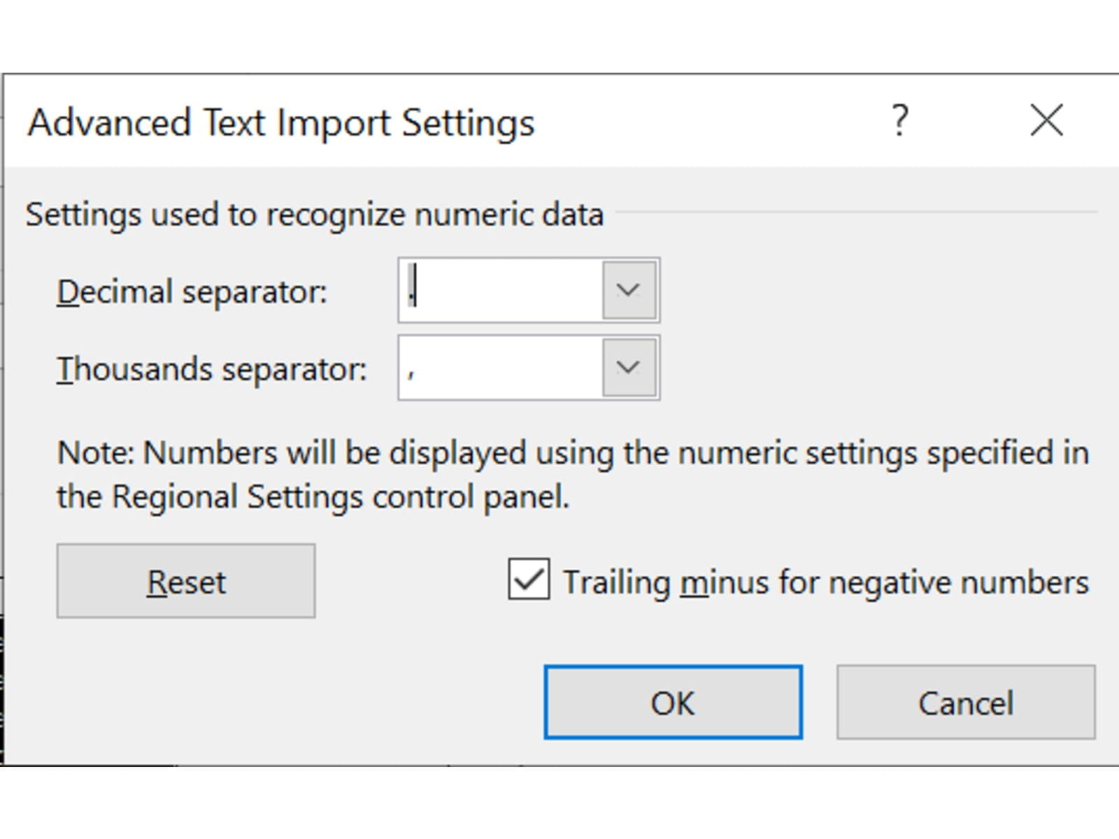
This lets you control how Excel interprets numeric data – useful if e.g. you have been supplied European number format data such as 4.123,06 and want to have Excel convert into UK / US standard. It can also handle trailing minus signs to convert e.g. 4,123.06- into a proper -4,123.06.
Once you are all done, Finish will output the completed data:
Note that Text to Columns is a programmatic step – it does not generate formulas or any kind of audit trail. If you are worried about errors in the transformation process, use the Destination box as described above to output the separated data separately from the original data.
Additional quirks
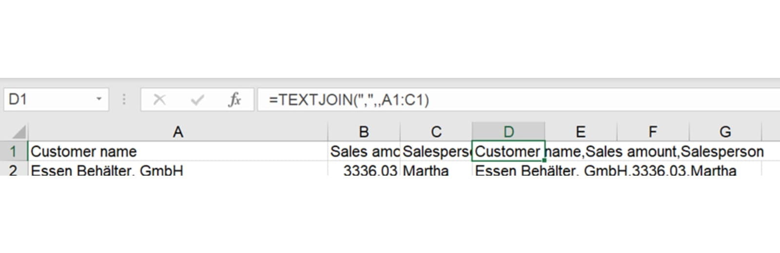
It’s worth noting that you can do essentially the reverse of Text to Columns using the TEXTJOIN function:
You can also automate the process of taking a set of data and splitting it using Power Query’s Split Column transformation:
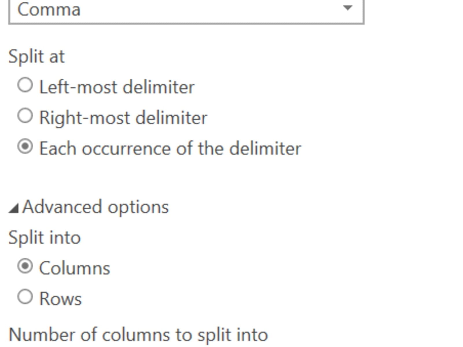
This has the advantage of being repeatable if you paste in new data later on.
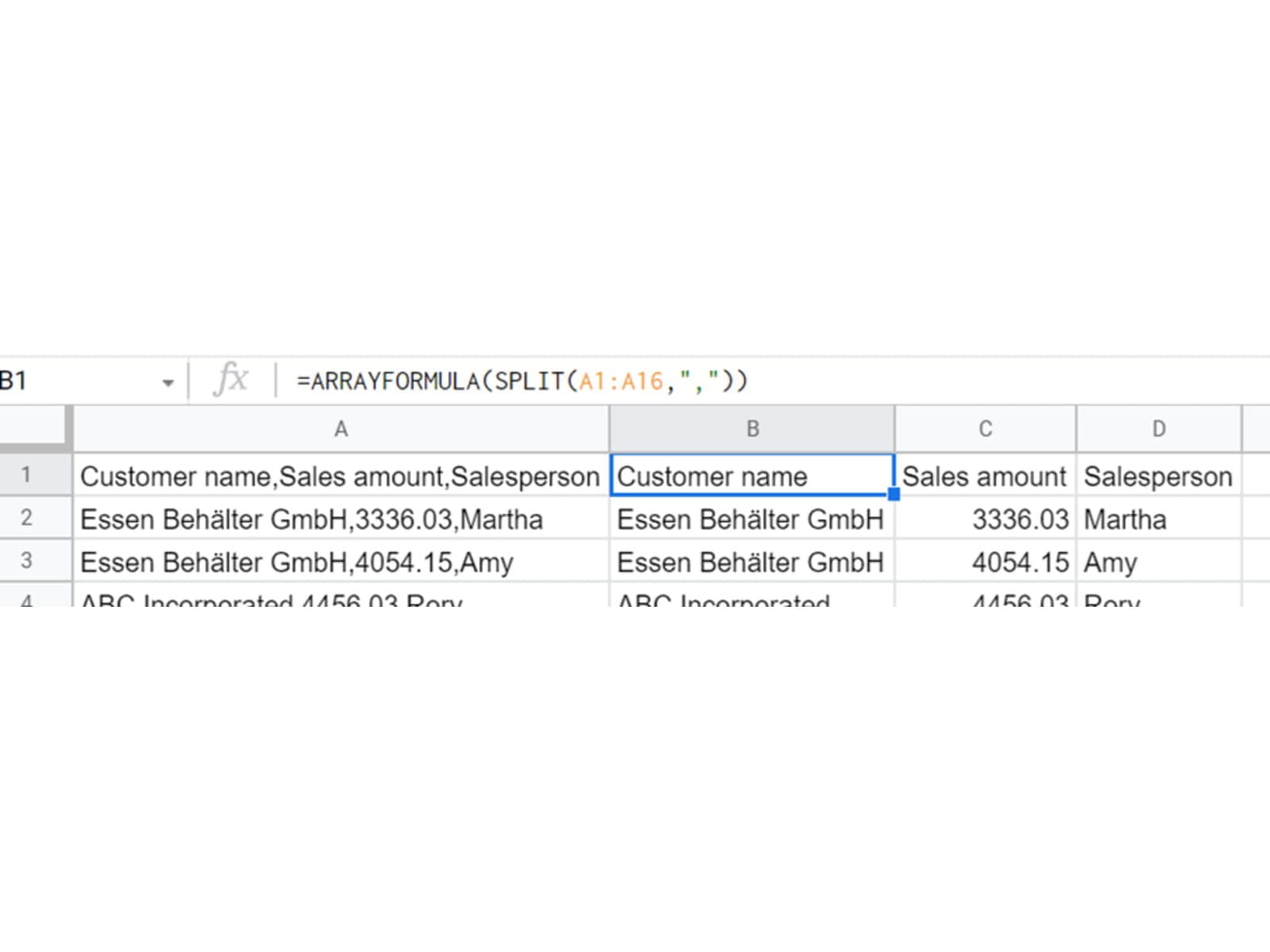
Finally, you might be wondering if it’s possible to split data this way formulaically – the answer is “No” with basic formula options, but Google Sheets does have a SPLIT function that can do it – although without the ability to declare a text qualifier:
Archive and Knowledge Base
This archive of Excel Community content from the ION platform will allow you to read the content of the articles but the functionality on the pages is limited. The ION search box, tags and navigation buttons on the archived pages will not work. Pages will load more slowly than a live website. You may be able to follow links to other articles but if this does not work, please return to the archive search. You can also search our Knowledge Base for access to all articles, new and archived, organised by topic.
