Power Query versus VBA – part 2

In the first part of this series, we compared the use of Power Query to Excel VBA to perform a calculation of the amount of Stamp Duty payable on a property transaction. If you have looked at both articles, you might have come to the conclusion that the Power Query approach was much more complicated. However, the Tip of the Week article simply sought to explain the VBA Select…Case statement and the figures used were hard coded into the VBA. In contrast, the Power Query example was based on the use of Excel Tables. This not only means that it is easy to change the values without needing to edit the calculation process itself, but it also makes it easy to adapt the process to cope with other similar calculations.

In this second part of the series, we will make our calculation process more general and show how it can be copied to other spreadsheets to create a more modular approach to the construction of spreadsheets.

This is a good example of the benefits of planning your spreadsheets in advance of starting to create them. Had we thought about the possibility of making the process more general, we could have given our Tables and columns more appropriate names from the start.

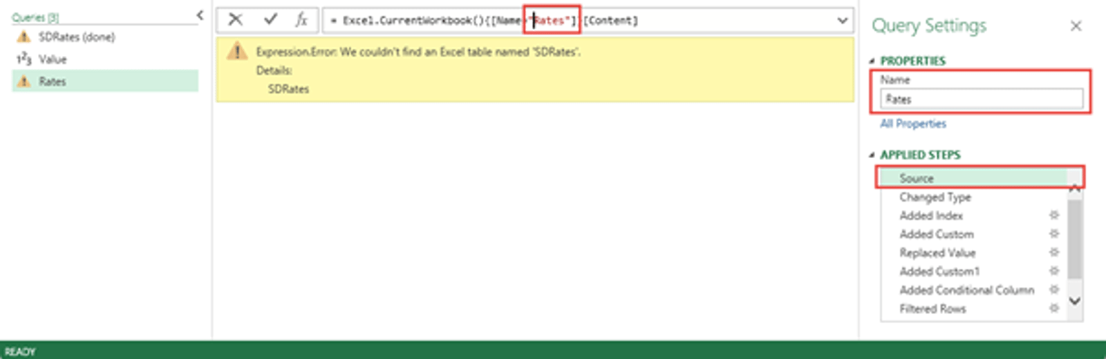
First of all, we will change the specific 'Price' title of our value column with the more general 'Value'. We will also change the name of the Table itself from Price to Value. We will need to adjust our queries as a result. As you can see, all our queries now show a warning symbol and, if we hover over a query in the Queries & Connections pane, we can see details of the error: "The column 'Price' of the table wasn't found":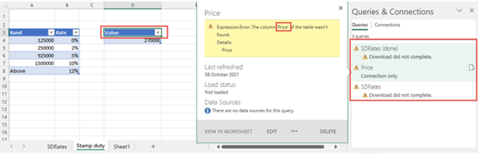

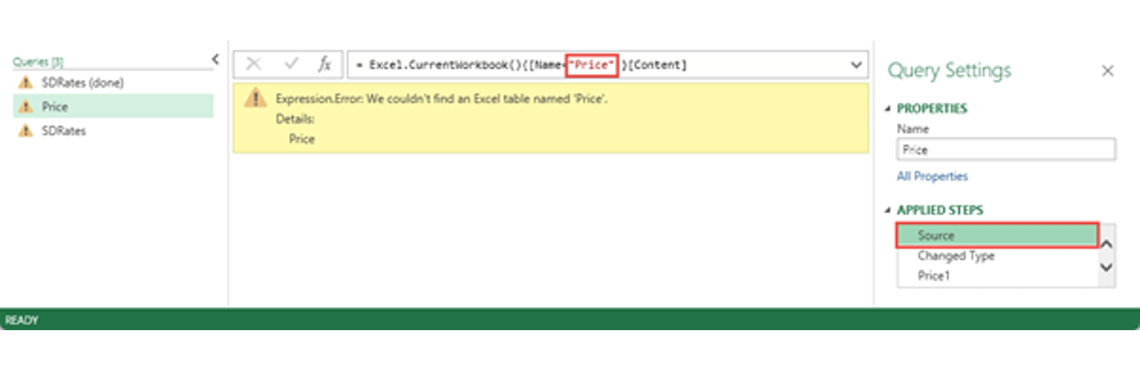
We need to right-click on our Price query and choose Edit to open the Power Query editor. We can then change 'Price' to 'Value' in the formula bar where necessary: first in the Source Step to refer to the Value Table:

Then next in the Changed Type Step to change the column name:

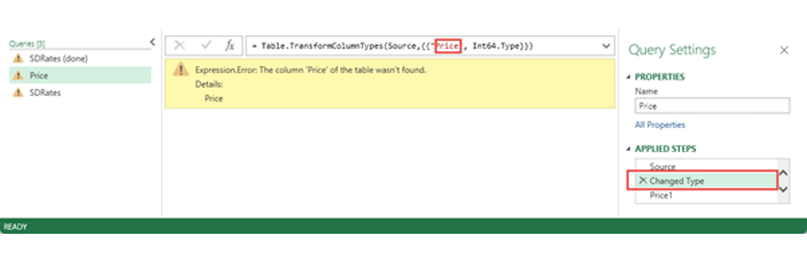
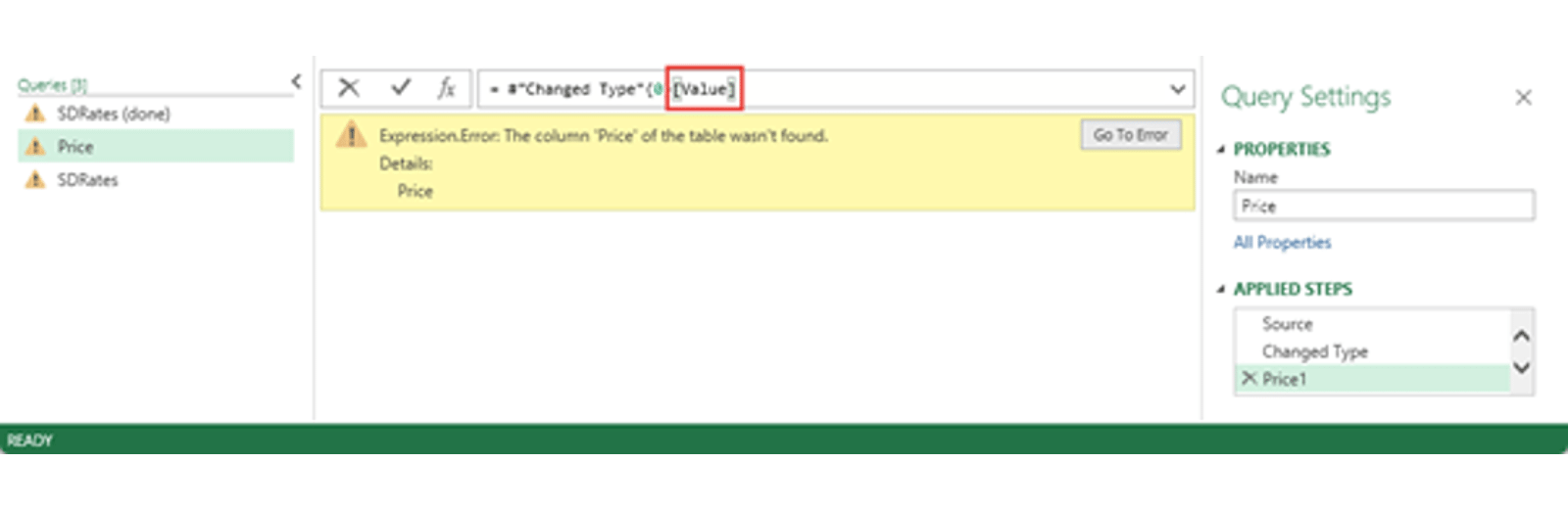
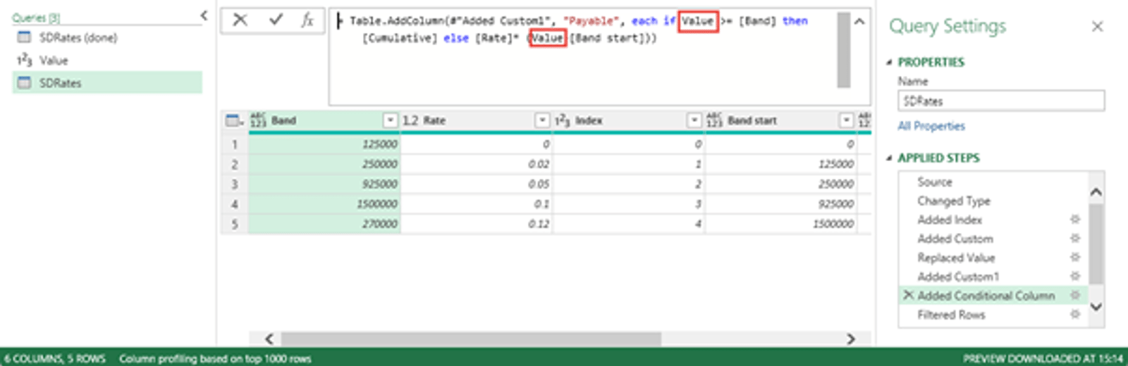
Subject to an Option setting, Power Query will automatically try and set the column data types of each of the columns of the Source table. This can often be useful, but it does mean that the query will refer to the names of all of the columns in the Source table before you have a chance to make any changes to the Source – for example, before deleting all of the unwanted columns. This increases the susceptibility of the query to errors caused by changes in the source data, possibly unnecessarily if the affected columns aren't even used. In our case, we only have one column and we obviously need to use it, so we won't delete our Changed Type step but will again change the step in the formula bar to replace "Price" with "Value". We will also need to make the same change in our final step. Here we see the step after we have changed [Price] to [Value]:

Our Price query now works as before, but it is still called Price. We can change the Name in the Query Settings Pane and this time, because we are making the change within the Power Query editor, the change will flow through into any other queries:

We also foolishly named our Bands and Rates table as SDRates so again we will change the Table name in Excel to just Rates and change the Source step and name of our SDRates query in the same way as we did for the Price query:

Fortunately, we have already given our columns the general names Band and Rate.

Of course, even without making these changes we could have changed our Band or Rate values and the changes would have been reflected in our calculation. Here we have changed our bands and rates and refreshed our result to show the recalculation:

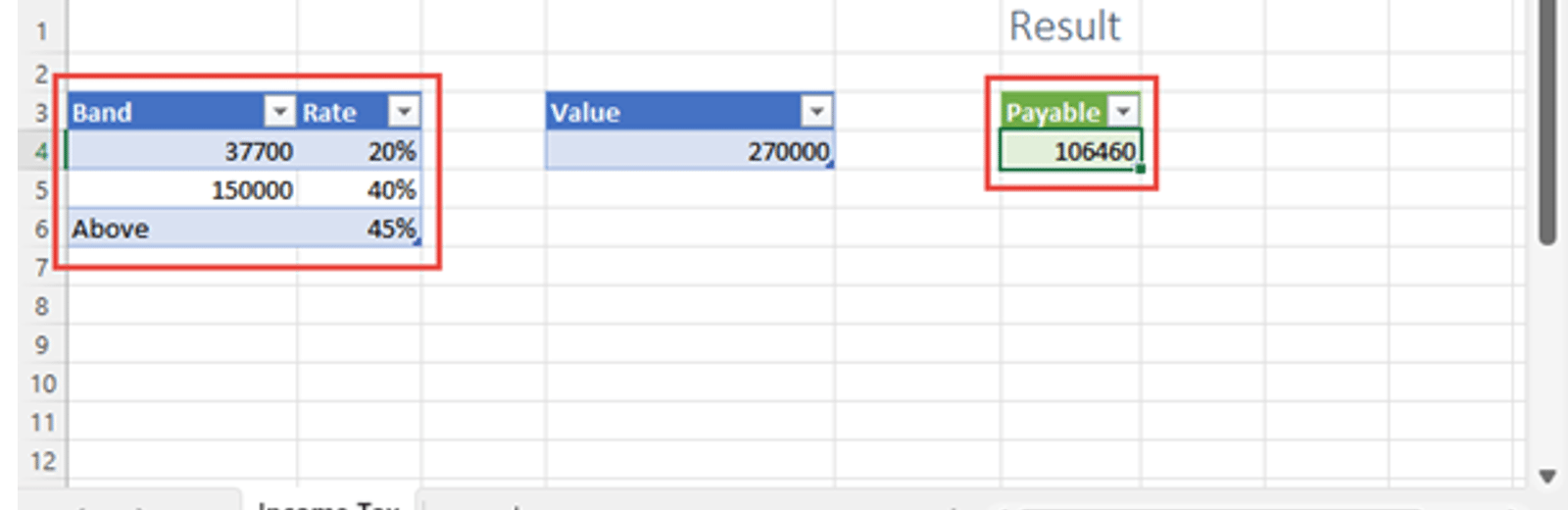
Further, we could change the number of rows in our Rates Table and, because Power Query works with tables and columns rather than individual cells, our calculation will still work as intended. Here's a tax calculation using the same Tables (note that this is a simplified example that assumes the Value is entered after the deduction of the appropriate personal allowance):

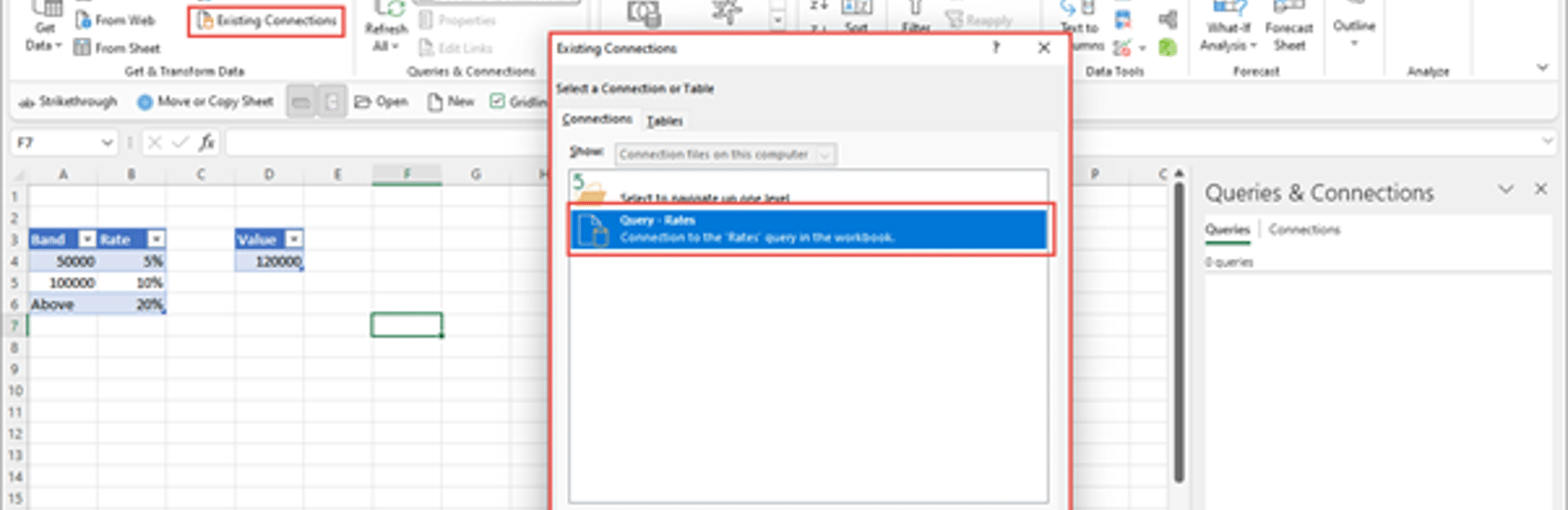
So, now we have a general way to calculate the amount payable based on a value and a Table of rates. We could just set this up as an Excel Template, but we could also treat our Power Query solution as a module that could be added to any Excel workbook. The workbook would need to contain a Table named Rates with a Band and Rate column and a Table named Value with a Value column. We could then simply copy the Rates query from the Queries & Connections pane of our existing workbook to the Queries & Connections pane of our new workbook and, as long as we had got our Table names and Table headings (including capitalisation) right, our calculation would be added to our new Workbook. Note that, because the Rates query depends on the Value query, we only need to copy the Rates query and the Value query will follow automatically. We can make the modularisation process a little more elegant. Rather than requiring the original workbook to be found and opened, and the correct query copied and pasted, we can right-click on our query and choose to Export Connection File… in order to save it to a chosen location. In our new workbook, we could then use the Data Ribbon tab, Get & Transform group, Existing Connections command to browse to a particular folder to import our previously exported connection:

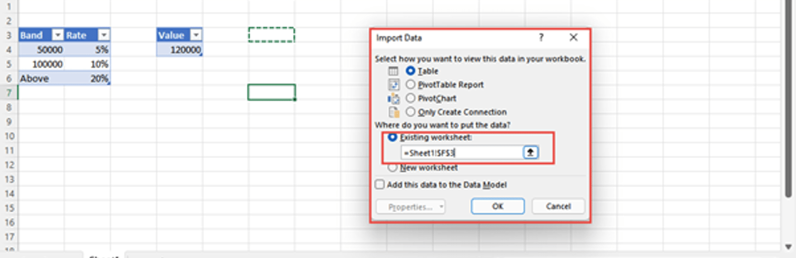
We can then choose where to place the result:

If we had a series of fully tested modular calculations that used Power Query, we could save them all to the same folder so our users could choose the calculation they needed from the list.