
Last time we saw how, in the new era of Dynamic Arrays, the SUM() function can be combined with the new FILTER() function to provide a more flexible way to calculate conditional aggregate values, potentially replacing the use of the likes of SUMIFS() and AVERAGEIFS(). This time we will take this idea a little further to show how we can construct an aggregate formula to include all the items that are matched against an entire list of criteria values.
Last time, we looked at how the combination of the SUM() function and the Dynamic Array FILTER() function could be a more flexible substitute for SUMIF(), SUMIFS() and the other similar conditional aggregate functions. In particular, we examined the use of Boolean logic to create combinations of AND and OR functions. In this article, we are going to see how we can use FILTER() to aggregate values that match one of many different criteria.
As we saw last time, we can use the + operator to include values that match either of two possible values, in the case of this example, the values in cells A3 or B3:
=SUM(FILTER(Invoices[Quantity],(Invoices[Country]=$A$3)+(Invoices[Country]=$B$3),0))
Were we to extend our list of criteria values, we could just add more + elements to our FILTER() include argument:
=SUM(FILTER(Invoices[Quantity],(Invoices[Country]=$A$3)+(Invoices[Country]=$B$3)+(Invoices[Country]=$C$3),0))
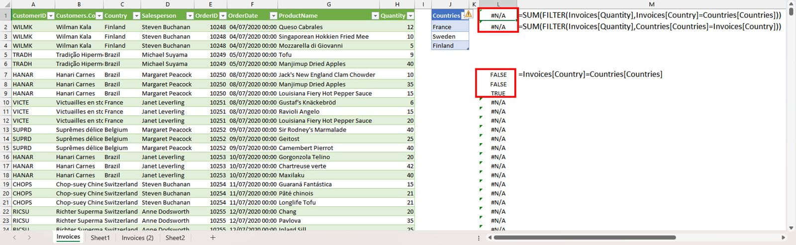
However, as we add further items to our list of possible matches, we would need to change our formula manually. It’s tempting to try comparing the column of countries in our Table to the list of criteria countries, but as you can see below, this results in a #N/A error, because, whichever way round we put our two ranges, if they don’t contain the same number of items, the ‘extra’ items will cause #N/A errors. In any case, the comparison is performed by just comparing each pair of items in order, rather than checking to see if any of the rows in one list match those in the other list. So, in the following example only the third item returns TRUE because each list contains ‘Finland’ as the third item:
To avoid this, we can use another of the FILTER() superpowers that we used in the previous article: the ability to manipulate ranges with functions. The MATCH() function allows the comparison of an item against a list of items and returns the position of each match in the list. This allows us to use MATCH() within our SUM(), FILTER() formula. However, this is not completely straightforward. First of all, it is important that you get the two ranges the right way round in the MATCH() function. We need our FILTER() ‘include’ argument to return TRUE or FALSE for each of the items in our Invoices Table. In the era of Dynamic Arrays, MATCH() will return a separate result for each item in the first. Lookup_value, argument. For our FILTER() formula to work correctly, we need the same number of items in the first two arguments. Accordingly, the first argument in MATCH() must refer to the column in our Invoices Table, rather than to our list of criteria countries:
=SUM(FILTER(Invoices[Quantity],MATCH(Invoices[Country],
Countries[Countries],0)))
This is not the end of the story. The above formula will return a #N/A error because MATCH() returns a position index number when there is a match and a #N/A error when there is no match. We need to convert each of these values into something that FILTER() will recognise as either TRUE or FALSE. There are different ways to achieve this, the IFERROR() function could be used with errors set to return 0:
=SUM(FILTER(Invoices[Quantity],IFERROR(MATCH(Invoices[Country],
Countries[Countries],0),0)))
This works because Excel treats 0 as FALSE and any number other than zero as TRUE, so the actual value that MATCH() returns where there is a match doesn’t matter.
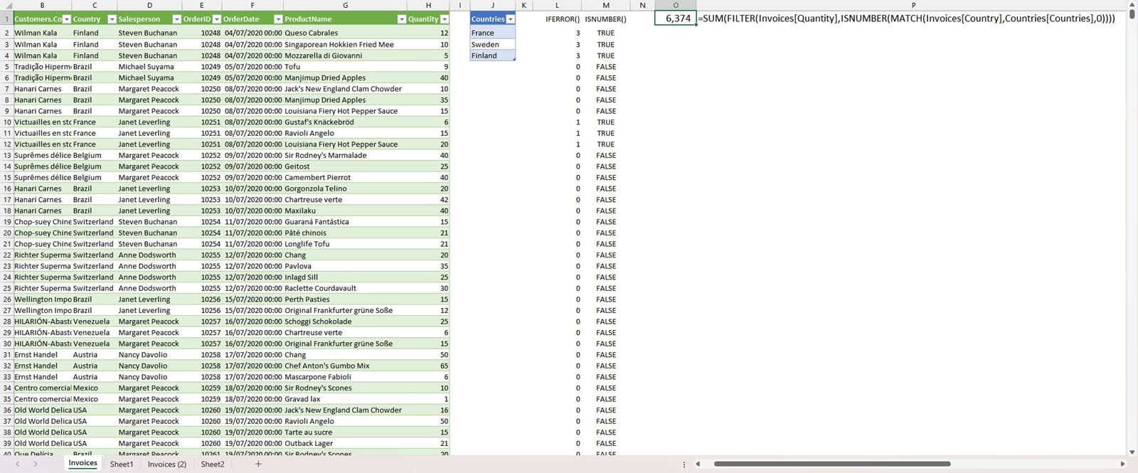
The preferred solution in several of the Excel Internet forums is to use the ISNUMBER() function. This is slightly simpler than using IFERROR() as it avoids the need to set a value for errors, instead it automatically treats errors as FALSE and matches as TRUE:
=SUM(FILTER(Invoices[Quantity],ISNUMBER(MATCH(Invoices[Country],
Countries[Countries],0))))
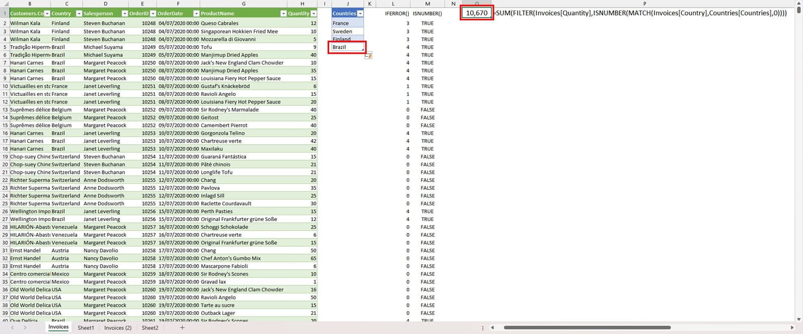
As we have set our list of countries up as an Excel Table, all we have to do is to add further countries in the Table to recalculate our value:
Links
The list of links included last time is still relevant, but with the addition of some articles on the MATCH() function and Excel’s error checking functions:
Archive and Knowledge Base
This archive of Excel Community content from the ION platform will allow you to read the content of the articles but the functionality on the pages is limited. The ION search box, tags and navigation buttons on the archived pages will not work. Pages will load more slowly than a live website. You may be able to follow links to other articles but if this does not work, please return to the archive search. You can also search our Knowledge Base for access to all articles, new and archived, organised by topic.
