Your Questions Answered #3 – Questions on the life-changing opportunities of Power Query?

• 'Why Power Query can change your life' - webinar recording now available 

The question

Could you just go over the basics of getting the original data into Power Query and then loading the end result back into the spreadsheet?

Answer part 1 – Data Sources

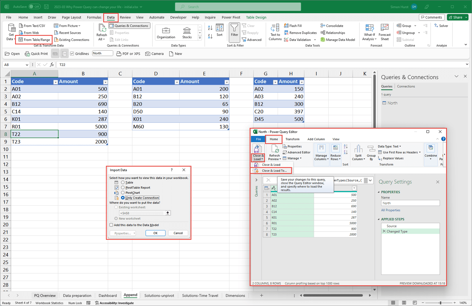
The Power Query tools are accessed from the Get & Transform Data group of the Data Ribbon tab. The main Get Data dropdown lists all the different data source categories as well as the command to use the old Excel Get External Data commands that are now known as the Legacy Wizards. Also, in the list of commands is Launch Power Query Editor which opens the Power Query editor directly. If you want to edit an existing query, it is usually easier to right-click on it in the Queries and Connections pane and choose Edit.

Towards the bottom of the list of commands is the Combine Queries command that allows multiple tables to be either appended (stacked vertically) or merged by linking two tables using common fields – a bit like using an Excel lookup function. To use either of the Combine Queries commands we first need to have the queries available in our Excel workbook.

To turn a block of cells in an Excel spreadsheet into a query we have to load it into the Power Query editor and then use one of the Close & Load options. If our data is already in an Excel Table, then we can click any cell in that Table and click on the From Table/Range command to read it straight into the Power Query editor to create a query with a name based on the original Table name. If, instead of being in a Table, the block of cells has an Excel Range Name allocated to it, then selecting the block of cells and using From Table/Range will create a query based on the cells referred to by the Range Name. If the chosen cells are neither an Excel Table nor a Range Name, then Excel will turn them into a Table as part of the process. More recently, it has also become possible to use a Dynamic Array as the source of a query.

When using anything as a Data Source, Excel is only interested in the data. Any values calculated using a formula will just be imported as the result values with no reference to the original calculation. Calculation columns can be added within the Power Query editor or by adding calculated columns to the output Table.

Answer part 2 – Output

The data is loaded back into Excel using the Close & Load command in the Close group of the Power Query editor Home Ribbon tab. The Close & Load button itself defaults to loading the output Table into a new worksheet (one of the Power Query options allows you to change this default). The dropdown includes the additional option to Close & Load to… This allows you to specify what sort of output you require (Table, PivotTable, PivotTable and PivotChart or just a Connection to be used for further processing). You can also specify whether the output should be put in a new worksheet or in an existing worksheet, specifying the top left-hand corner cell. You can also choose to Add this data to the Data Model:

Further questions and answers

How do you use one query as the starting point for a new query as you did when creating the grouped output table for the TreeMap chart in your dashboard?

A query can have another query as its Source so that when the output of the original query changes, those changes automatically feed into the second query. You do this by ‘Referencing’ the base query. This can be done in the Power Query editor window by right-clicking on the base query in the Queries pane at the left of the screen and choosing Reference. A new query is created with its source set to the name of the first query. Alternatively, you can right-click on the first query from the Queries & Connections pane at the right of the worksheet and choose Reference from there.

• Power Query - cascading queries

Is it possible to a use a previous Power Query in another workbook?

You can copy a query from the Queries & Connections pane in one workbook and paste it into the Queries & Connections pane of another workbook. If the copied query is dependent on other queries, these will also be copied automatically.

Can we append query in one dashboard and it refreshes the data in other spreadsheet if a link is created?

A query created in one workbook can be referenced directly from another workbook or the other workbook can reference an output Table created by a query. When refreshing links to a workbook, the link will retrieve the data from the last saved version of the file.

Could [Power Query] reference to onedrive/sharepoint folders, or would they have to be local?

Yes, Power Query can reference folders or files on OneDrive or SharePoint but to work properly you need to link to the online version of the file, rather than the local copy:

• https://learn.microsoft.com/en-us/power-query/sharepoint-onedrive-files?source=recommendations 

Is this very much like Power BI?

Yes, Power Query is basically the data acquisition component of Power BI. The functionality is very similar but not always identical.

If you made the vstack formula into a table it would automatically update wouldn’t it? Would that total error problem be solved if you just used the name range rather than the standard?

This question related to the section of the webinar that compared Dynamic Arrays and Power Query output tables. I failed to mention that one of the big (current) drawbacks of Dynamic Arrays is that they can’t be used to create an Excel Table. It is possible to avoid some of the problems of referring to Dynamic Arrays by using the # operator. A reference to the top-left hand corner cell of a Dynamic Array, with the # suffix, will return the entire array rather than the single cell:

• Dynamic Arrays - limitations of # (note that, since this article was written, an Excel update has enabled charts to link directly to a Dynamic Array).

How can you use Power Query to remove duplicates?

In the Power Query editor, you can right-click on one or more selected columns and use Remove Duplicates to delete any rows where the values are identical for all the columns selected. In the example in the webinar, we only wanted to remove entries that were the same for all columns, so we selected all columns before using Remove Duplicates.

How does Power Query affect Excel workbook file sizes?

The size of a workbook that contains Power Queries substantially depends on the data loaded to the workbook as Tables. A workbook linked to a file that contains 80Mb of data will be of minimal size until the data is loaded back into the workbook. If the data is loaded unchanged, the file will be very similar in size to the original file. If the data is filtered or summarised into a few hundred or thousand rows before loading to the workbook, the file size will be much smaller than the original.

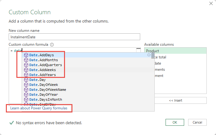
How do you find the equivalent Power Query formula for an Excel formula? Can you use power query to show the date of the instalment if you split the instalments over a year, say rather than in the next x months? What function would you use to add different time lags for cash receipts for different customers e.g. invoiced in Jan but cash receipt will come in say 2/3/4 months?  Can I use the Date.Addmonth that you just used?

When typing a formula in the Power Query editor, Excel will display a list of functions that match what you type. So, if you know that you want to add periods to a date, you could type ‘Date’ and Power Query would display a list of Date functions that you could use. In this example, you would find a list of Date.Add…. functions to add different periods:

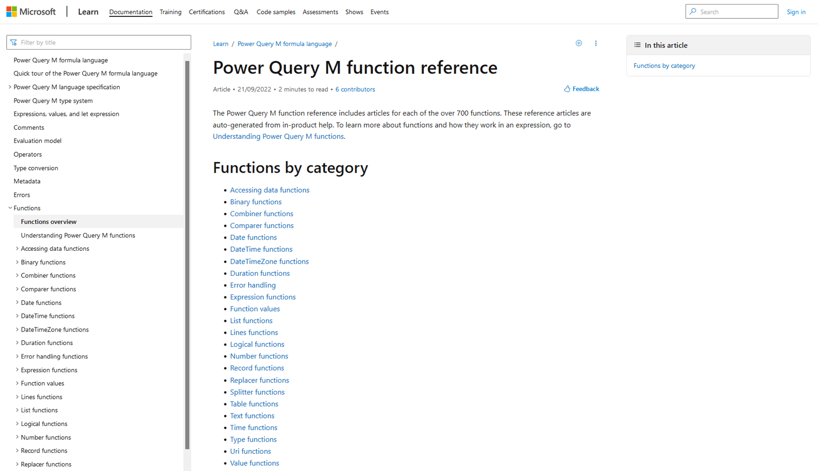
The dialog also includes a link to display the online Power Query Function Reference which lists all the available Power Query by category with full descriptions and help:

If you needed to add different periods for different customers, you could create a separate customer table containing a field to hold the period value and merge the tables:

• Christmas special - the spreadsheet gift that keeps on giving - part 8

Is there a way to show the age of dates before 1900 in years rather than days in PowerQuery?

Sort of. You can get an approximate conversion by just dividing the number of days by 365.25 to allow for most leap years. This is not perfect as it obviously depends on when the leap years fall and how many years that are divisible by 4, but are not leap years, are included. To get an exact answer, you would need to deconstruct the date into day, month and year and then use a series of IF() comparisons to work out the exact difference between the two dates. Regrettably, Power Query doesn’t seem to have (yet) an equivalent of the hidden Excel DATEDIF() function.

If it was purely the number of years (without worrying about additional months and days) you could use Date.Year() to extract the year from each date and then subtract one from the other, with an additional conditional formula to subtract one if the day/month portion of the later date was before the same portion of the earlier date. Searching the Internet will reveal all sorts of alternative methods of performing the calculation.

I missed why you added an index column when showing the unpivot ability? Also, instead of unpivoting / pivoting to remove the empty March column, couldn't you just hit "Remove" on that column?

These questions refer to an example that used Power Query to remove a blank column. We used a simple table that included separate columns for results from January, February and March. There were no results for March, so we wanted to create a version of our original table that omitted the March column entirely. To answer the easier of the two questions first, just removing the March column would have always removed the March column, rather than whichever column was empty. The reason to add the index is twofold: it ensures that each row is unique so that the Pivot operation doesn’t group the individual values; it also enables us to keep the output rows in the same sort order as the original table.

Is there a way to set up a query that gets an output linked to a month? I am looking at producing a monthly sales report showing current month vs budget and prior year from a data table.

Yes, one way to do this would be to use a cell in the worksheet that allowed the user to choose the month that they wanted to see, then Power Query could use this value to filter the output table accordingly:

• Power Query - using individual cell values