Your Questions Answered #9 – What is the purpose of # when using dynamic arrays?

• ‘Dynamic Arrays refreshed’ recording now available

Questions by attendees fell broadly into two areas: general concepts about dynamic arrays; and specific questions about dynamic array functions. These have been grouped and answered below.

General Concepts

The Question

Is the use of dynamic arrays automatic (i.e., I do not have to specify to excel I now wish to use dynamic arrays)?

Answer

Yes, dynamic arrays are built into the calculation engine in Excel, so there is no need or requirement to switch them on.

Dynamic arrays are available in Excel 2019 and subscription versions of Excel (Microsoft 365). Users on earlier versions of Excel will not have access to Dynamic Arrays.

The question

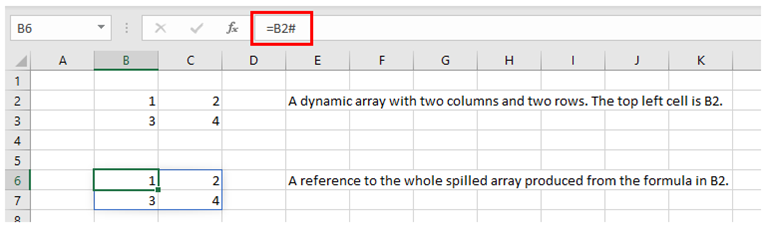
What is the purpose of #? I have never come across it before.

Answer

The # operator allows you to refer to a dynamic array. This syntax ensures that the range reference will automatically update if the dynamic array changes in size.

The question

Can the dynamic array apply horizontally (to columns) as well as vertical (to rows)?

Answer

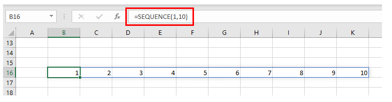
Yes, dynamic arrays can be a single row, a single column, or a rectangular range containing multiple rows and columns.

Here is a horizontal dynamic array created from the SEQUENCE function producing 1 row and 10 columns.

The question

In "old" excel, we had to use the square brackets to denote an array formula by pressing “Control Shift Enter” when exiting a cell. Is this still required for old-style arrays?

Answer

For backwards compatibility the old style “Control Shift Enter” arrays still work and can be entered in the same way.

However dynamic arrays completely supersede the functionality of the old-style arrays and are much more powerful and easier to use.

The question

Does a dynamic array take up less memory or resources than copying a formula down?

Answer

Probably, as Excel only has to remember one formula instead of multiple copies of a formula.

However you are unlikely to notice a difference in performance unless you are working with very large amounts of data.

The question

Using power pivot enables you to double click to see underlying source data - is there any way to use similar functionality with dynamic arrays?

Answer

Dynamic arrays do not offer this double click functionality but, as with all formulas in Excel, you can select the range inputs to the formula by using the “trace precedents” feature. This can be achieved by selecting anywhere in the array and using the keyboard shortcut Ctrl + [.

Formula Examples

The question

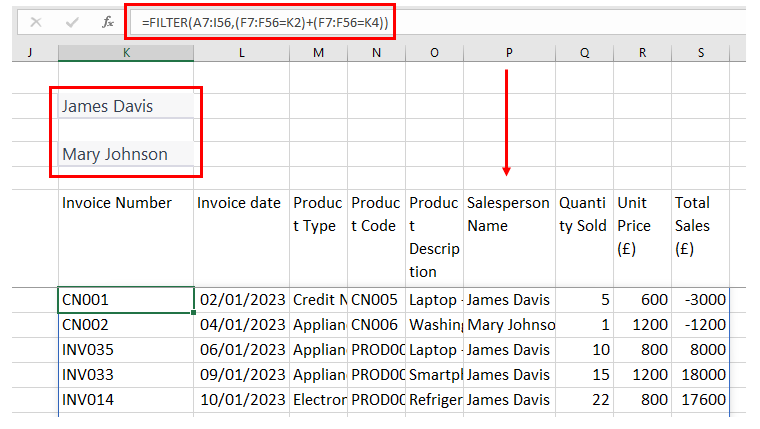
In the example presented in the webinar, on the sales data can you select two salespeople?

Answer

It is not possible to select multiple items from a single data validation drop down. However we can create a copy of the data validation drop down in another cell so that we have two separate drop downs to choose from.

These can then be incorporated into the filter function as two separate criteria.

=FILTER( array , (range = criteria 1) + (range = criteria 2) )

By putting our criteria in brackets we can then add them together to return rows where either condition is true.

A similar technique can be used where the requirement is to filter by multiple criteria (i.e., where they are both true rather than where only one criteria is true). In this scenario, replacing the addition + operator with the multiplication * operator will achieve the desired result.

The question

When using the FILTER function, does inserting an additional column in the source data impact the FILTER summary?

Answer

Yes, the dynamic array will automatically expand to bring in the additional column and this will be reflected in the output.

The question

How does one add an extra calculated column to a spilled array (for example, adding a %age calculation to the array of total sales by salesman)?

Answer

A percentage calculation column could be achieved with the following formula.

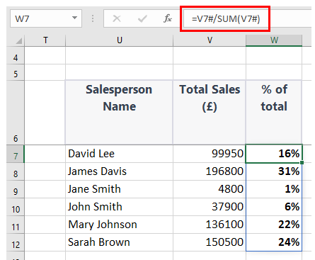
Here the numerator is referencing the whole dynamic array in column V. That creates the spilling behaviour of the output in column W. The denominator is the total of the dynamic array in column V and will divide each value by that amount. The usual number formatting options have been applied to present the output in column W as a percentage.

The question

Can you show us how to use the Sequence formula to get a list of month-end dates?

Answer

The following formula will produce the next twelve month ends.

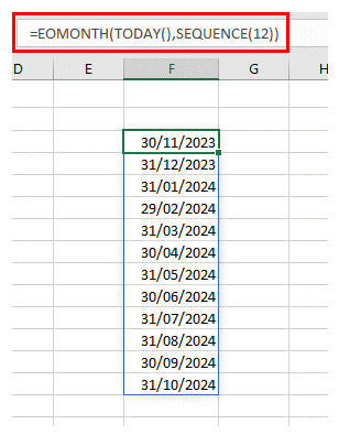
This can be adapted as required by manipulating the arguments in the SEQUENCE function. For example, if you wanted it to run from the current month you could replace SEQUENCE(12) with SEQUENCE(12,,0).

The question

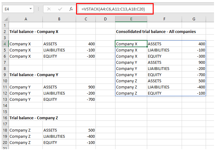
I did not understand VSTACK and its purpose. Can you explain this in more detail?

Answer

VSTACK allows you to join multiple arrays together by arranging them vertically. A practical example might be if you have multiple company trial balances that need to be brought together into a single larger table for a group consolidation.

The question

Can you think of a practical application of EXPAND?

Answer

EXPAND could be used to ensure that dynamic arrays are the same size before joining them together with either VSTACK or HSTACK.

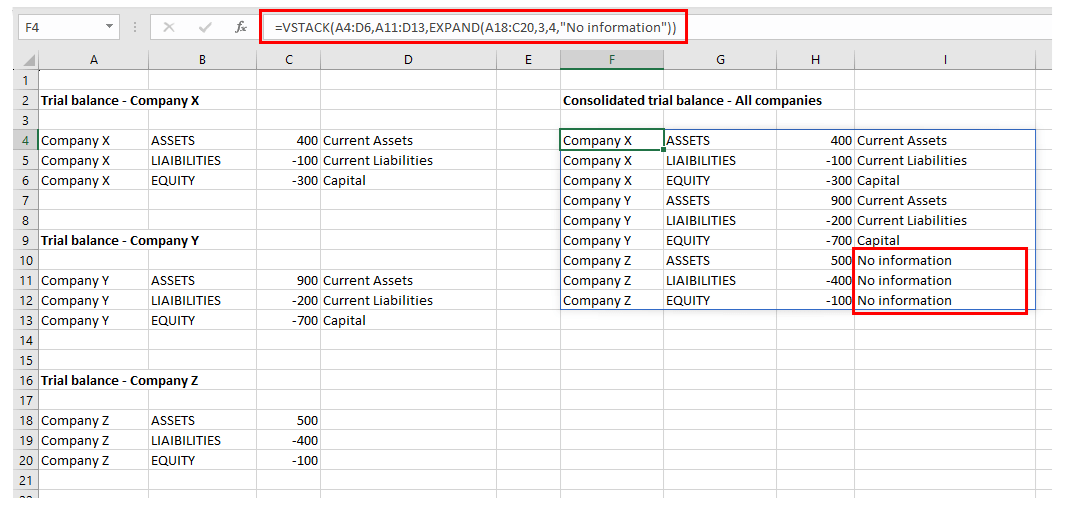
Building on the VSTACK consolidation example above we could imagine a scenario where there is an additional column with more detailed nominal information for Company X and Company Y, but this information is not available for Company Z.

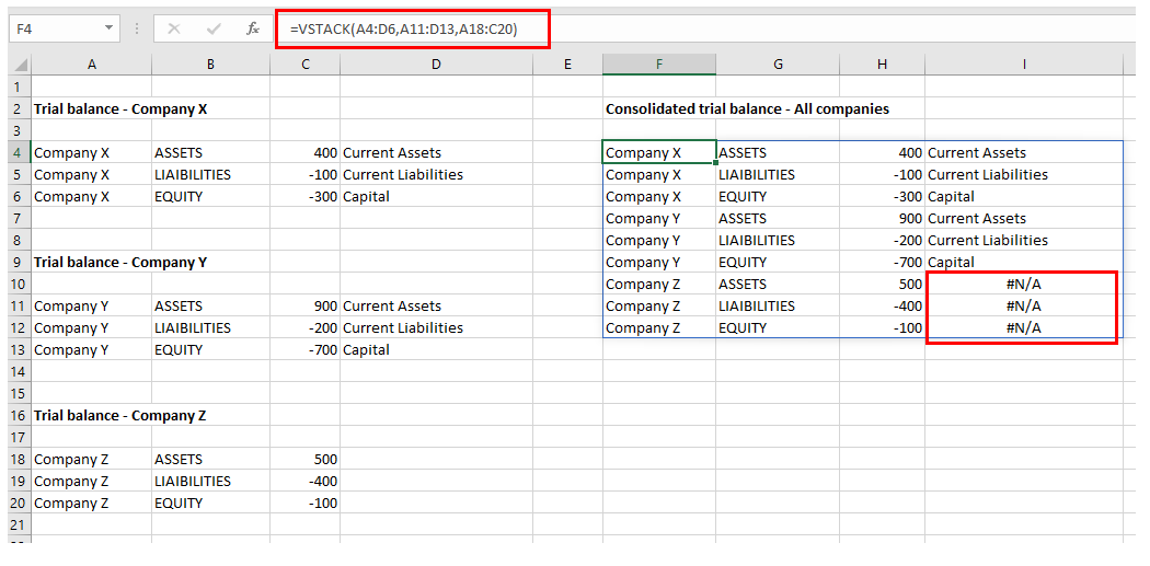
Notice how we have errors in the bottom right-hand corner of our consolidation where the data is missing. This scenario can be handled more gracefully with the EXPAND function as that gives us the option to choose what to “pad” our missing data with.